Regression describes the process of estimating the exact value of an object. Unlike classification – where we try to predict a distinct class (e.g. dog, cat, or human) – in a regression task we try to predict a particular value on the number line.
For example, if you estimate the age of a person to be 57 years based on their height, hair color, and wrinkles on their skin, you perform a regression task. Similarly, if you estimate how much a car of a particular brand, color, with a few scratches and a given mileage should cost, you perform a regression task. In other words, you use the characteristics of an object to estimate its value.
While the better term for this process might be ‘value estimation’, there is a reason why we call it ‘regression’. In the 19th century, Sir Francis Galton, a Victorian-era polymath, observed that the descendants of tall people tended to be less tall - in other words, they were growing to a more average height; he called this a ‘regression towards the mean’. The same was true for the descendants of small people. Therefore if you knew the average height of a person at that time and if you were taller than that, you knew that your descendants would probably be smaller than you.
In modern terms, particularly in the context of machine learning, regression means that each characteristic of an object can be used to estimate the value of that object. So looking again at the two original examples, knowing that a person has an adult height, white hair and a lot of wrinkles will allow you to estimate this person is probably ‘old’. Or if a car has a lot of mileage, scratches, and is made by a mediocre brand, its value will be rather low.
In both cases, you used the characteristics about an object to estimate its value. It’s important to note here that in the context of regression, its value can be any continuous feature you choose. For example, we could have also tried to respectively estimate the height or number of wrinkles, or the car’s mileage from the remaining information in the data.
Machine-based regression
In a previous article, we learned that the task of regression belongs to the machine learning category of supervised learning. In supervised learning, we try to predict an outcome value (also called the target value) based on the input data.
In a regression approach, this outcome prediction is a continuous value – i.e. a number on the number line, such as 3’120 CHF, 72.3kg, or 22 months. This stands in contrast to a classification approach, where the outcome prediction is a discrete label, such as ‘dog’, ‘cat’, ‘fish’, or just simply ‘yes’ or ‘no’.
Artificial intelligence performing regression can be encountered on numerous occasions. It is known for predicting tomorrow’s temperature based on past recordings, for predicting a person’s annual income based on their education, age and ethnicity, as well as being useful to predict the yield and demand of a dairy farm based on a multitude of characteristics from the market.
How humans learn to estimate a value
To better explain how a machine learns to estimate the value of an object, let’s first reflect on how we humans would do this. For this, let’s imagine you are the owner of six ice cream shops throughout Lausanne.
Drawing on years of experience, you have developed an intuition for what is driving demand. While there are multiple factors, you boil it down to four important points:
- The more people that are passing by your shop, the higher the sales.
- The warmer it is outside, the more likely people will buy ice cream.
- People are more likely to buy ice cream during the weekend and less so during work days.
- The closer people are to the lake, the more they think of ice cream.
Having intuition is great, but to manage a business you need numbers. So you spend time analyzing the books, looking at sales and collecting additional information from the weather station. Finally, you are able to quantify the exact numbers behind the four key points:
- 2% of all people passing by your shops will buy an ice cream.
- For every 5°C temperature increase outside, your sales will go up by 50%.
- On weekends, you sell double the ice cream than during any work day.
- The two shops that are closest to the lake sell 2.5 times more ice cream than others much further away.
Your intuition and bookkeeping skills allow you to develop a good estimation of the demand for ice cream in your shops – perfect! However, recently you realized that your estimations are not always ideal: some days you have too much ice cream, on others you don’t have not enough. This creates waste and missed opportunities. Your goal is clear: you want to have a better estimate of the actual demand for ice cream so that you are as close to the actual number as possible.
Thankfully, having amassed data over all these years, you are able to combine your love for ice cream and statistics, and perform a regression analysis. In other words, you try to find the optimal way to combine the information you have about your shops in order to predict the overall demand of ice cream.
To start with, let’s take a look at two features – people passing by and temperature – and plot them against the ice cream demand. Each red point in the following plot shows the sales at a particular shop on a specific day.
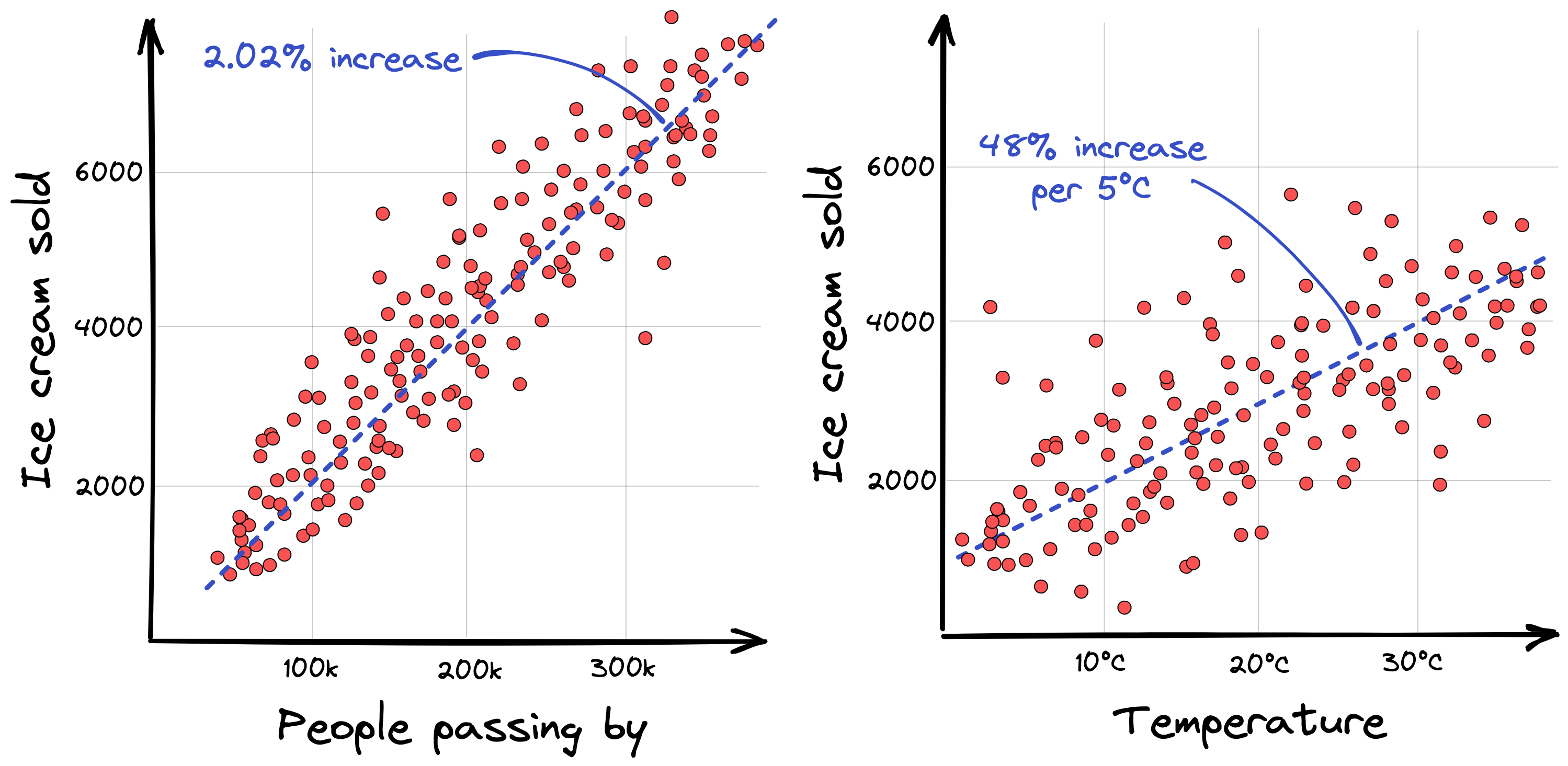
What we can see is that the relationship between people passing by or temperature outside and the target value ‘ice cream sold’ is extremely linear, shown by the blue dashed line. This means the more people that pass by, or the warmer it gets, the more ice creams are sold.1
However, in the temperature plot the points are spread much wider, indicating that the linear relationship is less pronounced. But in the case of temperature, this makes sense: people might buy more ice cream on a very sunny day at 8°C than they would on a very rainy day at 32°C. Therefore knowing more about rainfall or cloud coverage might help to estimate the actual ice cream demand even better.
And what about the other two features from our list, day of the week and distance to lake? How do they relate to the target value ice cream sold?
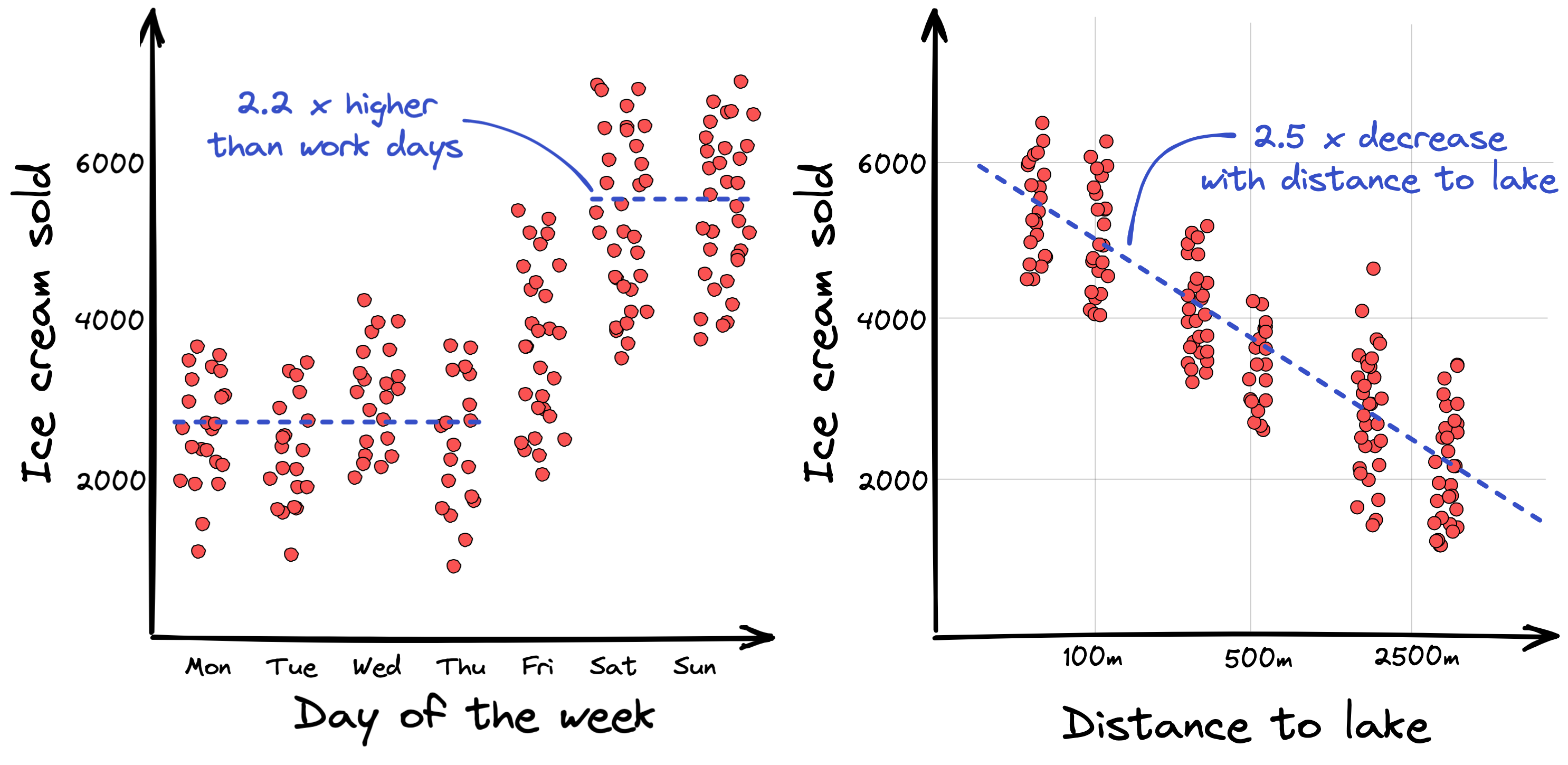
Looking at the feature day of the week, we can see that there is more to it than just having “double the sales during the weekend”. Wednesdays show slightly higher sales than other work days, except for Fridays which seem to be in between work days and weekends. This is certainly something you could use to improve your estimations. Meanwhile, with regards to distance to lake, everything looks as expected.
And that’s it! That’s how we would do a regression analysis, more or less. There are of course some statistical approaches that can help to estimate all of these factors at once, but what we eventually end up with are four individual parameters (or coefficients) – one for each feature in our dataset – that tell us how to combine them to get the correct prediction for ice cream being sold.
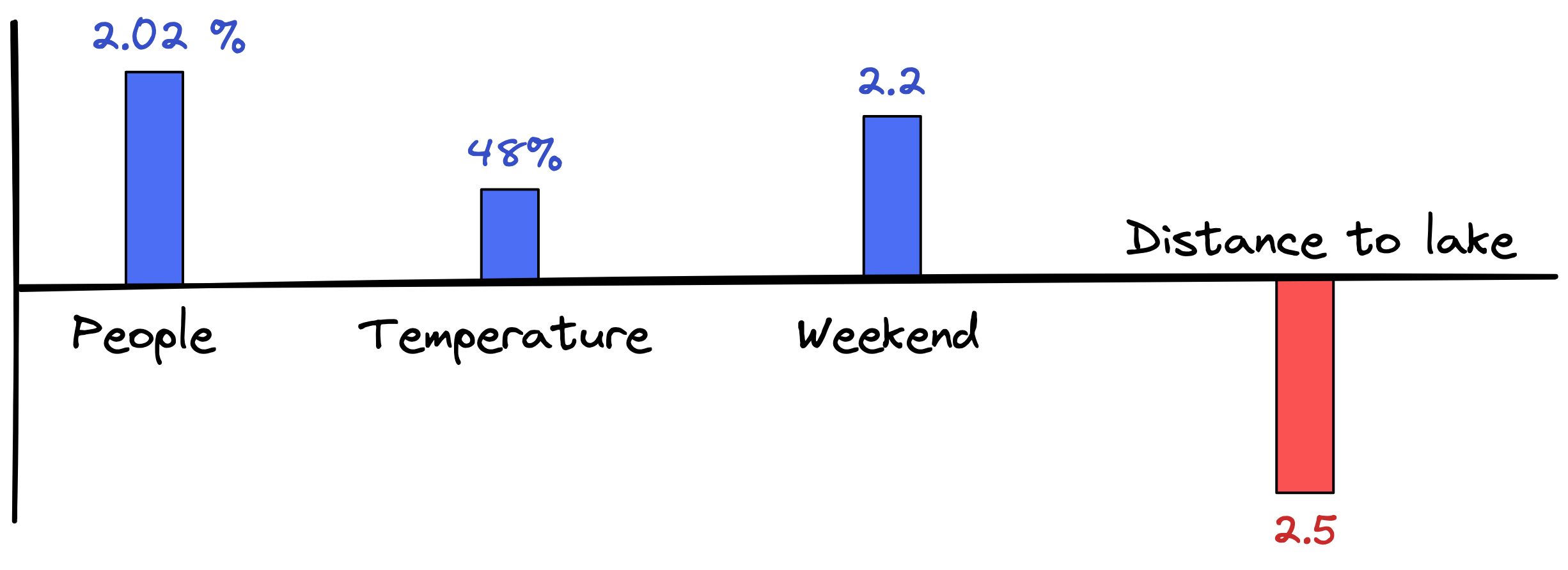
These are the four parameters we got from our regression analysis. The taller the bar, the more influential the parameter is for the prediction. And if the influence is positive – i.e. the more people that pass by, the more ice cream that is sold – then the bar is positive (shown here in blue). Otherwise it is negative (shown here in red). For example, the further away from the lake the shop is, the less ice cream that’s sold.
Together, these four parameters represent your model and are able to estimate how much ice cream you will sell in a shop on a given day. If you know the number of people passing by, the temperature, if it’s a weekend or not, and you know the distance of the shop to the lake, then you can compute a reasonable estimate of the demand.
Regression is nothing new
There is of course more nuance to this, but overall that’s how we humans would do it if we could approach it manually – look at the data and extract a parameter for each feature. You probably did this kind of exercise in school, called linear regression.
We actually perform this kind of regression analysis all the time. If you want to guess how tall a building is, you might try to estimate it by imagining how many average-sized adults you could put on top of each other to reach the height of the building. For this you would need to know the parameter for the height of an average person, plus the distance from you to the building.
Or when you estimate how much spaghetti to cook for lunch, you will consider how many people are coming, how many of them are children, if the children had a snack around 10am or if they are super hungry after sport, plus whether you want to make extra for the evening, and so forth. All of these are parameters that allow you to achieve the best prediction possible given the information at hand.
As another example, imagine you want to buy a new house and want to estimate the price of the house yourself. You might consider the size of the living area, the number of bathrooms, if it has a garden or not (and its size), where the house is located, and if it is close to supermarkets and schools. While you might not have clear numbers for each of these parameters, all of these elements factor into the estimation of the house price. In other words, all of these model parameters help to predict what the house is worth.
What makes regression difficult?
The approach shown in the ice cream example above generally works very well. However, as we have seen, having additional information about the weather – such as rainfall and cloud coverage, or considering Wednesday and Fridays as their own special days – could potentially help us to make even better predictions. So let’s adapt our model to include these additional features and look again at the model parameters:
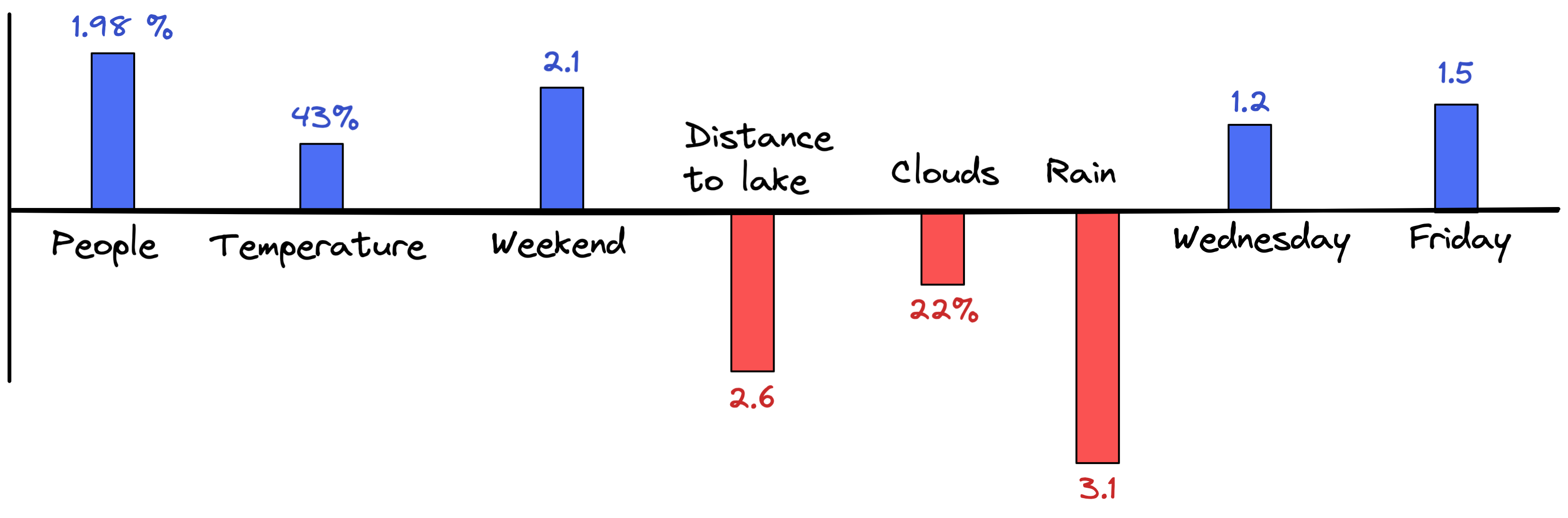
The four new parameters (clouds, rain, Wednesday and Friday) are more or less what we would expect. However, it is important to highlight that the inclusion of these new features into our model also changed the parameters for our initial four features: people, temperature, weekend, and distance to lake. So every time we change our dataset by adding days or adding features, the model parameters need to be estimated once more as the outcome will be slightly different.
Most of the time, having more and more additional information about your shops’ sales activity and the world around them will help you to make better estimates of the ice cream demand. For example, sales numbers might go up slightly if the day is also a holiday, but only if it’s during the week, otherwise it stays stable. And if there is a carnival in town, sales numbers go dramatically down even if there are more people in the city, because on those occasions people might prefer cotton candy over ice cream.
Keep in mind the goal of any such model is to exploit the patterns in the dataset to help with the prediction. But for every new parameter you add to your model, numerous new patterns can be investigated – some of them useful, some of them not. And figuring out which ones are which is not always straightforward, as patterns might also interact with each other in ways that are too complex to grasp just by looking at the data. Furthermore, some of these patterns might actually be too subtle to see with the naked eye. And so, once more, if the task becomes too complex, too time-consuming, or too daunting to do by hand, we can ask a machine for help.
How machines learn to estimate a value
Let’s now look at the same task as before and see how a machine could learn to predict the demand for ice cream. However, to be able to better show a few important points, let’s increase the number of parameters in our model to 25.
So now we have 25 different data features that we would like to use for our prediction. How would an AI go about solving this task?
Linear regression models
Actually, an AI could solve this task in pretty much the same way we humans would – by performing a linear regression. To briefly explain a linear regression, we multiply our data with the model parameters and add everything up to get our prediction value. The tricky part is to find the best optimal parameters to perform this prediction.
Let’s see what would happen if an AI doesn’t use any special tricks and tries to estimate the 25 parameters the way humans would. One potential solution could look like this:
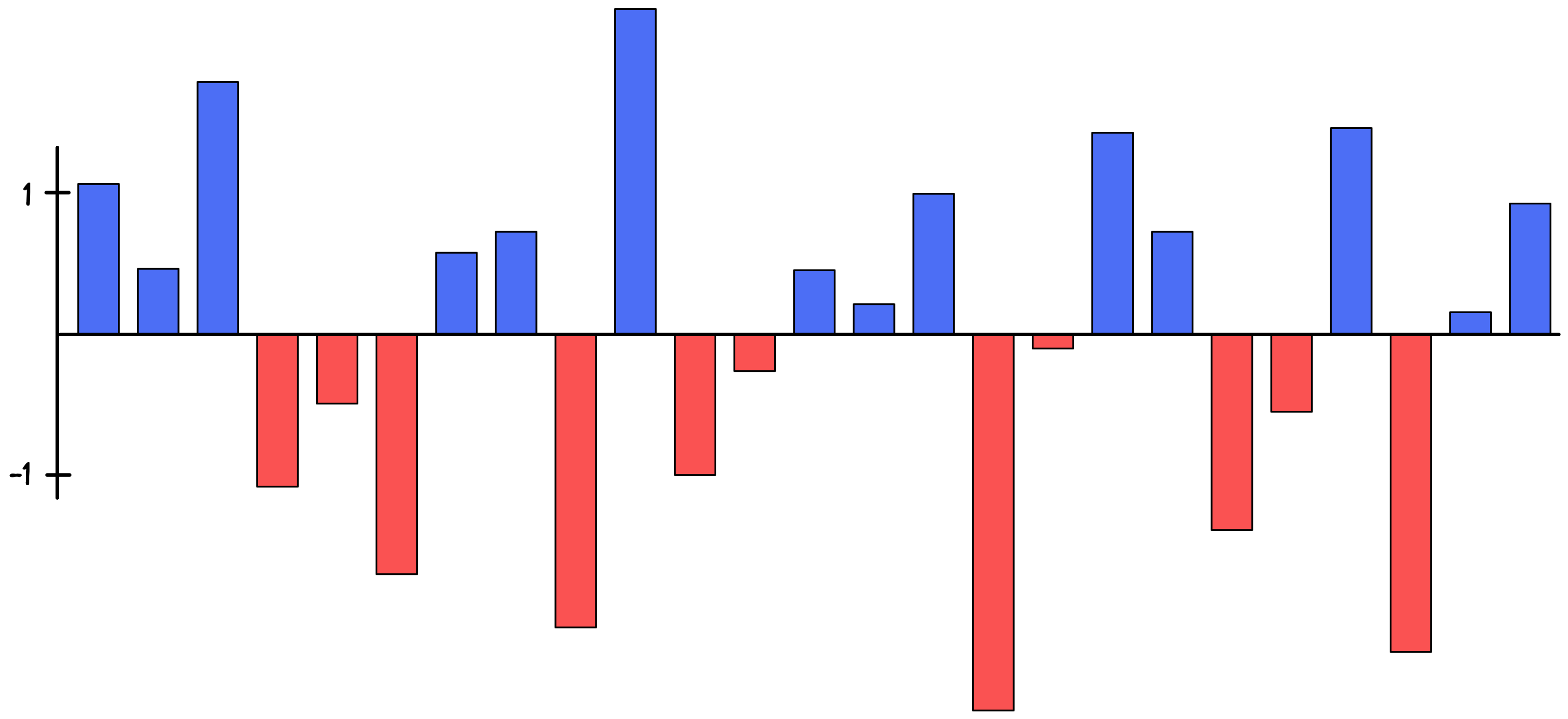
While these parameters might look reasonable and are capable of predicting sales numbers rather well, they might not be the best ones to consider in general. As we also hinted at, this might just be one of a potentially infinite number of parameter solutions, and not all of them lead to a useful model.
The reason for this is due to potentially high dependencies between some parameters. For example, in the previous figure we estimated the parameters for people and rain to be 1.98% and -3.1. However, an equally likely parameter solution could be 198% and -310 – meaning the 100 times bigger influence on the first parameter might be compensated by a 100 times bigger influence by the second parameter.
In a normal linear regression model, there might not be anything stopping these amplifications, which means model parameters can get out of hand and become very big. This is also what we can observe in the figure above.
The problem is while these huge parameters might work well for the dataset the model was trained on, they can make it very difficult to apply the model to any new data after the training, because huge parameters also mean that the model is very sensitive to small changes in the dataset. So the moment a data point is slightly different than usual, the model prediction will be a long way off. Thus controlling the size of these parameters is something the AI can help us with.
The tool that allows the AI to control this explosion of parameters is called regularization. The more regularization we apply to the model, the smaller these parameters need to stay; the less regularization, the bigger the parameters can become. Finding the right balance between enough and not too much is exactly what the AI tries to find.
By looking at numerous different model versions, each with a different amount of regularization, the AI can learn which version to choose so that the model performs well not just on the training dataset, but also on any other test dataset it might encounter later on. Visualizing the 25 parameters of such a regularized model could look something like this:
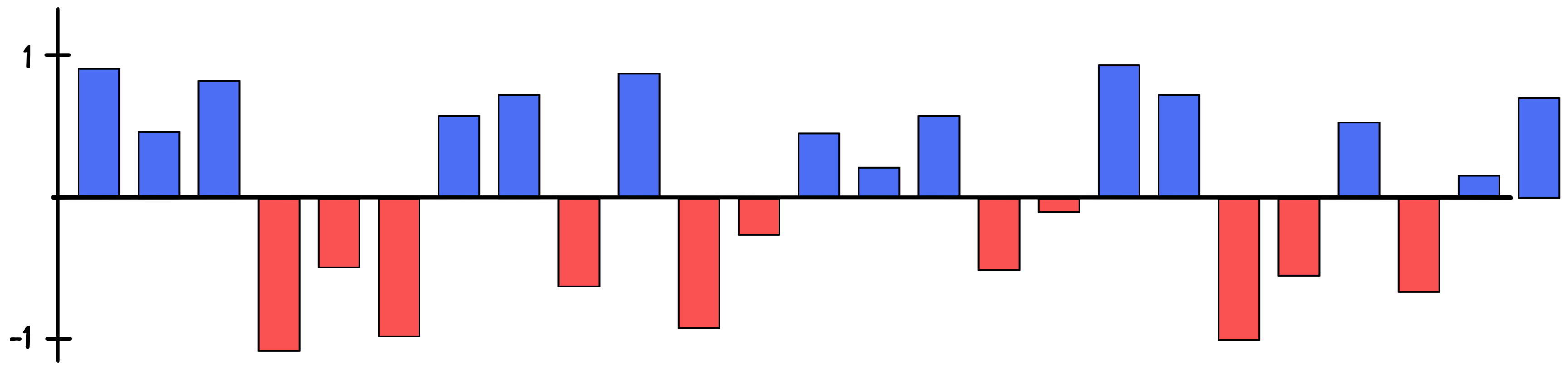
As we can see, these parameters are now much smaller than the ones in the previous illustration. But this is not the only way an AI could solve this linear regression task.
An alternative way of controlling parameter dependencies is to restrict the models to as few parameters as possible. This means that even though the model contains 25 potential parameters, the AI should try to find a way to put as many of these parameters to zero so that only the most influential ones survive. And as before, the AI will do some tricks and create multiple different models, all of them with more or less parameters set to zero. It will then investigate which of these models works best for the data it was trained on, as well as for other datasets it is tested on.
A potential solution for this task is shown in the next figure:
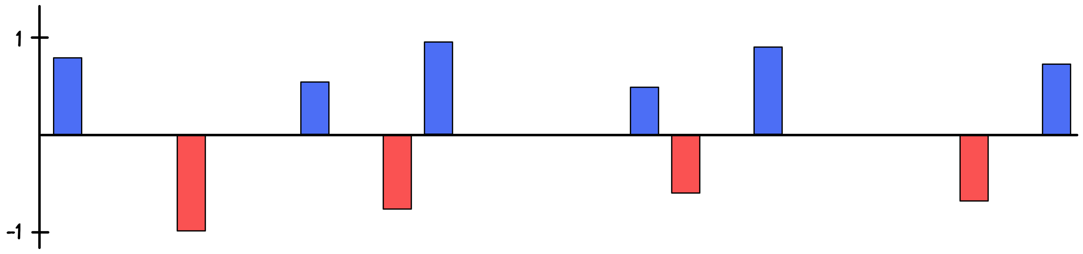
Controlling the height of the parameters and trying to set as many of them to zero as possible are just two of the ways an AI can optimize a regression model. There are of course many more. What is important to take with you is that the goal of the AI is to create many different versions of a model, all with different amounts of regularization and parameter controls, and then try to learn which of these models leads to the most optimal solution.2
Other regression models
Linear regression models are of course not the only way an AI can do regression. For example, you can also use deep learning and create an artificial neural network to perform a regression task. But going into the details of how exactly this works, or which other more classical machine learning models exist to perform regression, is outside the scope of this article. What is important to highlight is that most Classification models (if not all of them), can also be used to perform a regression task (and vice versa).
For example, in the Classification article we learned that a k-nearest-neighbors classifier algorithm assigns each point in a dataset the same label as its closest k neighbors. So if six out of 10 closest neighbors around a specific data point are all labeled ‘cat’, then this new and unknown point would also be predicted to have the label ‘cat’.
And so in a similar way, a k-nearest-neighbors regressor can look at the closest k neighbors to estimate the value you want to predict – usually by computing the average of all of these neighbors. For example, if you see a group of six teenagers and you know the age of five of them, taking their average age to predict the age of the sixth person would be a reasonable process. That’s how an AI can take a classification model and use it as a regression model.
-
A linear relationship isn’t always positive for both features. It can also be the case that one goes up while the other goes down. The important part is that they always change in equal parts, e.g. the first one goes up by 2.4 for every 6.5 the other one goes down. ↩
-
For more about this, check out our description of the ‘all-at-once training approach’ from the Machine Learning article. ↩