Classification describes the process of assigning an observation to one distinct category. For example, imagine you go for a walk in the forest and see something moving 40 metres ahead of you. Assuming that it’s an animal – it could be a deer, squirrel, dog, etc. – what you try to do is classify the observation, i.e. assign it the right label.
Based on the available input data – the size and colour of the animal, as well as the location and time of year, for example – you probably conclude that the animal you see is a deer. You’ve already seen other deers in this forest, moreover the animal has the height and shape of a deer. In other words, you came to this conclusion because you have already seen similar animals with similar characteristics in similar locations. Essentially, you have learned through past experiences what a deer looks like.
But what if once you get closer, you realize this is actually a new art installation of a deer made out of wood? This will probably change how you classify a distant observation in the forest the next time you encounter something far away. In other words, your internal model of deers and other forest animals is updated; you’ve learned to improve your object classification by making mistakes.
But how did we know that it could be a deer (or a dog) in the first place? Well, humans are incredible visual learners and we are able to transfer our knowledge from one experience to another. A toddler who has never seen a tiger before, for example, will be able to identify one in a photo after being shown a cartoon tiger just once beforehand.
For a long time, AIs struggled with such a seemingly simple task. Even today, they are still not adept at doing such knowledge ‘transfer’, also called ‘transfer learning’.
Machine-based classification
In the previous article, we learned that the task of classification belongs to the machine learning category of supervised learning. In supervised learning, we try to predict an outcome label based on available input data.
In a classification approach, this outcome prediction is a discrete label – such as ‘dog’, ‘cat’, or just simply ‘yes’ or ‘no’. This stands in contrast to a regression approach, where the outcome prediction is a continuous value, i.e. a number on the number line (e.g. 3’120 CHF, 72.3 kg, 22 months).
Artificial intelligence performing classifications can be encountered on numerous occasions. Such AIs are famous for detecting if an incoming email is ‘spam’ or ‘not spam’; if a breast X-ray image of a patient shows a cancer or not; or just to identify what kind of object can be seen in a specific image. For example: does the image contain a pedestrian, your friend Steve, or simply a dog?
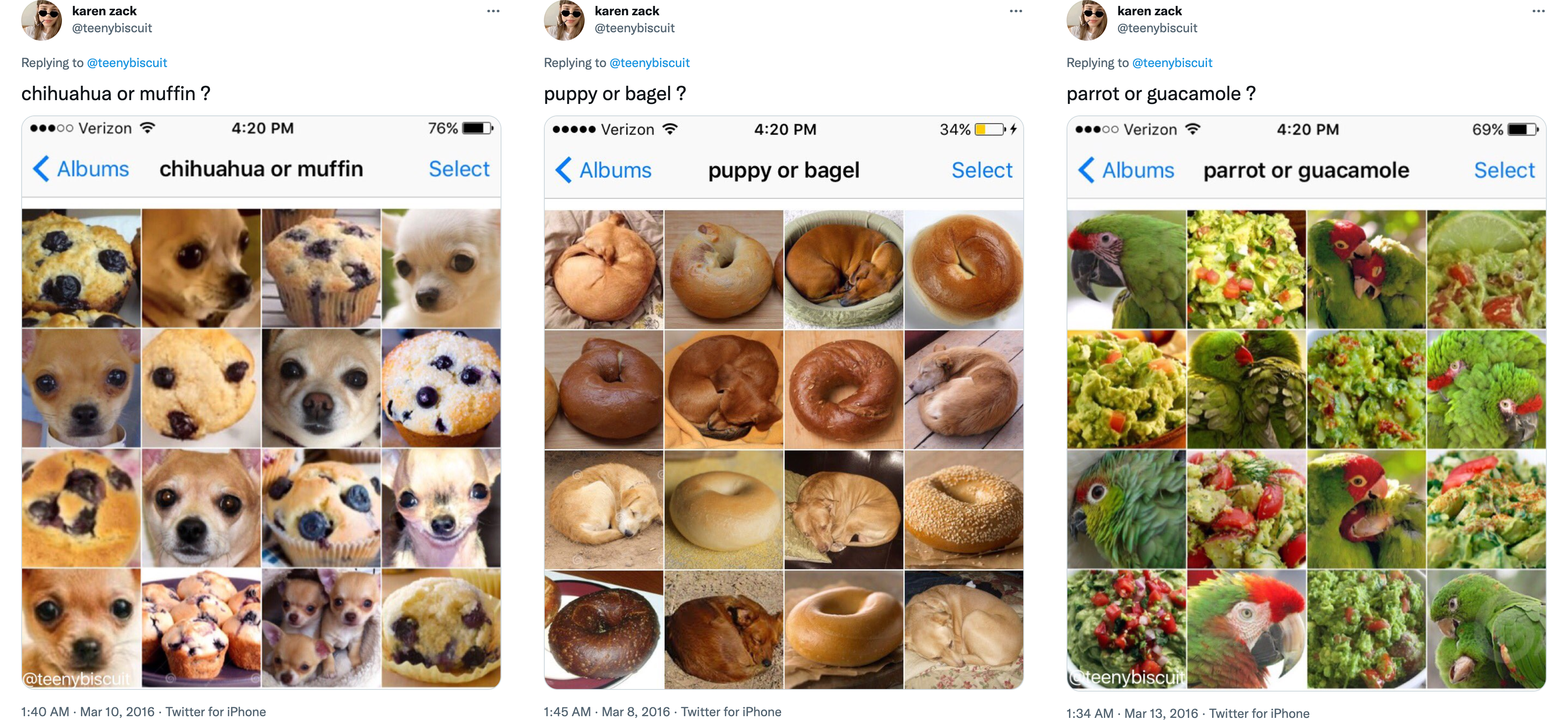
The last example might seem easy to do for us humans, but keep in mind that such a classification task should work for all possible images that exist in the world. For example, how easy and quickly can you decide if the following tweets contain (left) a muffin or a chihuahua, (middle) a puppy or a bagel, (right) or a parrot or guacamole?
If you think that those are the only strange and unusual combinations, think again – there are many more.
How humans learn to classify objects
To better explain how a machine learns to classify an object, let’s first also reflect on how humans do this. Let’s imagine we are researchers located close to the South Pole, studying the three penguin species: chinstrap, gentoo and adélie.
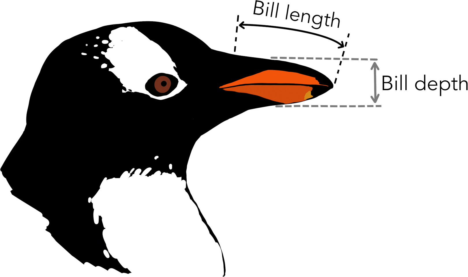
We are lucky enough to measure hundreds of penguins and record characteristics that we think might be useful to classify them – in other words, be able to identify their species based on the data we record.1 Two of these characteristics are the length and the depth of their bill.

Is this information already enough to correctly identify the species of a specimen? Well, as a first step, let’s take the data of all penguins and plot them in a figure, with the bill length on the horizontal axis and the bill depth on the vertical axis.
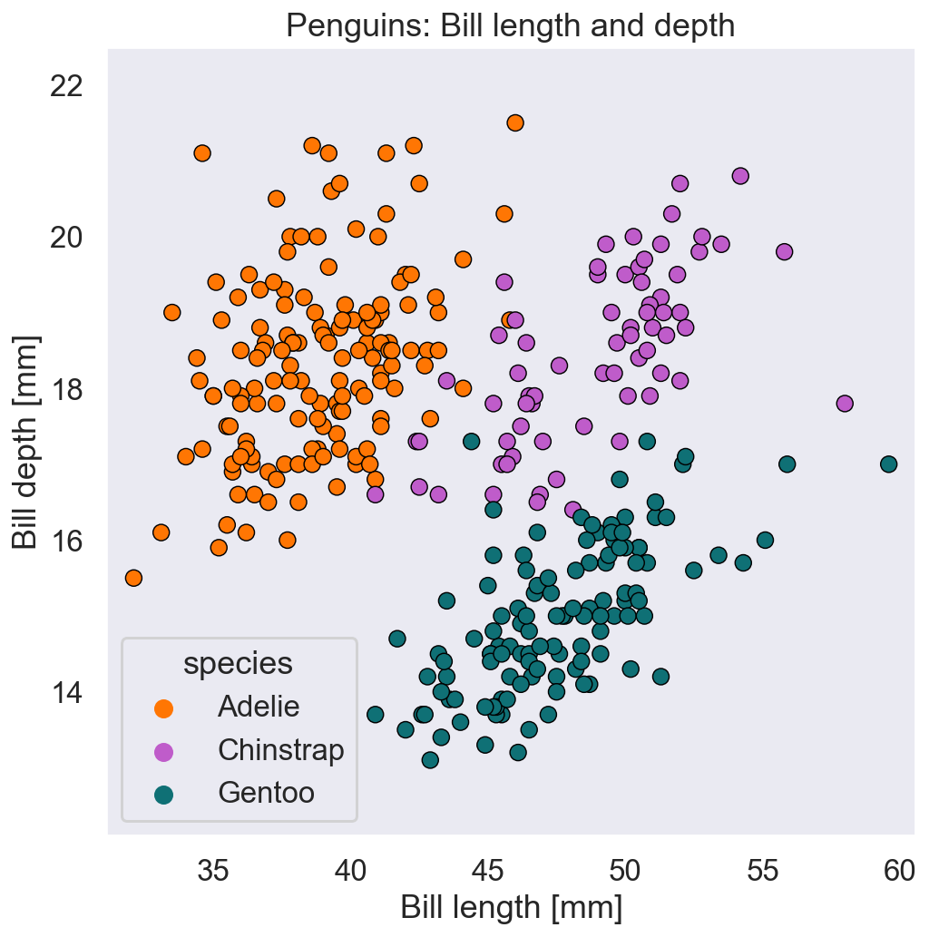
Looking at this figure, yes: it seems that the three species (shown in three different colors) can be classified depending on their bill length and depth. But what if we recorded a new specimen, of which we only know the bill length and depth, but not yet the species? How would we go about classifying the new observation?
The best idea is probably to identify specific regions in this figure where the likelihood that a penguin belongs to one species is much higher than the other two. It could look something like this:
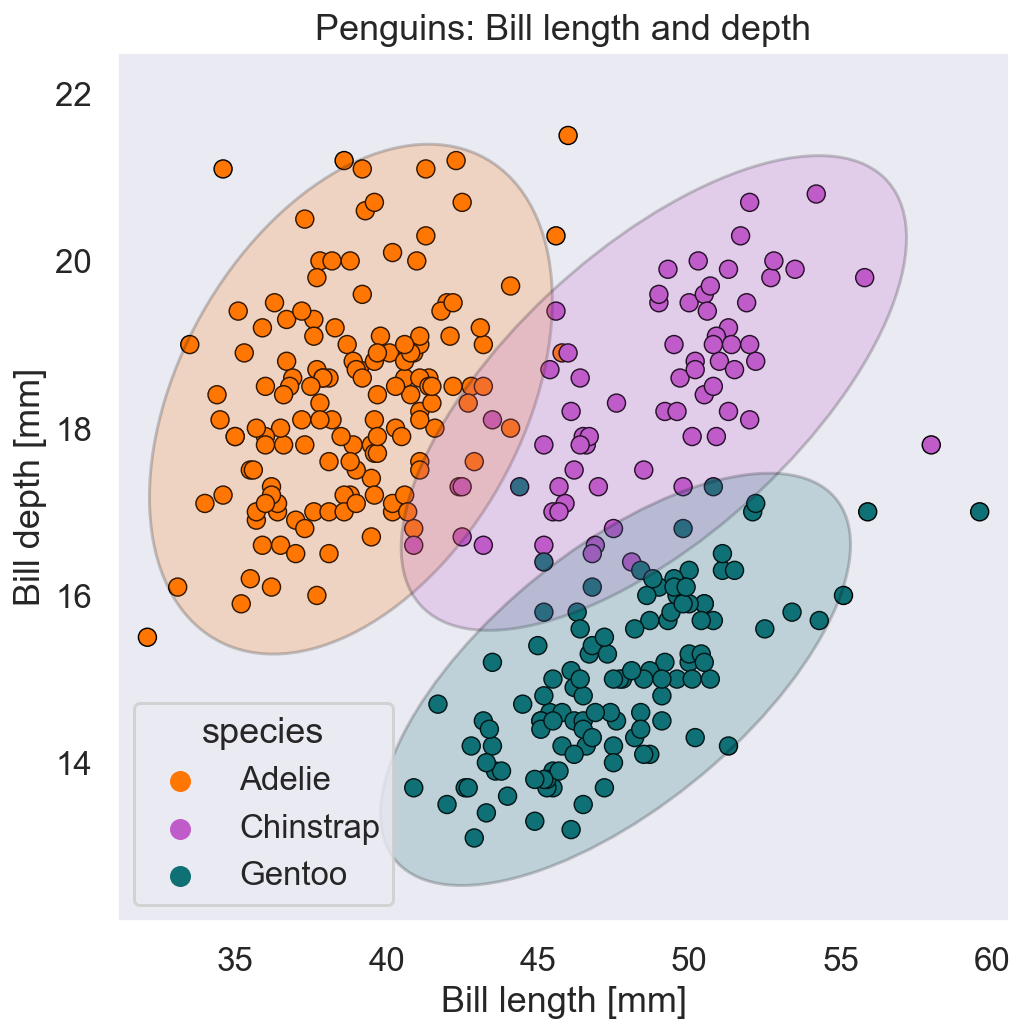
New observations that fall into either of these colored regions most likely belong to the species that the color indicates. However, as you can see, not all observations are within these regions – some regions are overlapping and some observations are in the ‘wrong’ regions. But these are not necessarily mistakes, they are more likely just uncertainties in our data that arise from reducing the penguins to only two characteristics: the length and depth of their bill.
Even a penguin specialist that knows the bill data for each penguin by heart would struggle to identify the species of a new penguin based on these two features alone, thus we should not expect this from a machine either. In fact, as we will see later, we would prefer that the machine makes a few minor mistakes during the training of the model, so that in return it will be better prepared for the uncertainty of the real world.
How machines learn to classify objects
Let’s now look at this same problem and see how a machine would learn to classify the three penguin species according to their bill length and depth. And to better understand the nuanced characteristics of how the machine learns, let’s explore three different model families: decision trees, k-nearest neighbors and support vector machines.
The goal of this exploration is not to teach you the intricate details of these AI models, but to show you (in a hopefully intuitive way) that there are many different ways a machine can go about classifying objects – with some of them being more, and others less, relatable to us humans.
Decision tree – the ‘if-then-else’ rules approach
Decision trees are very useful machine learning models because they are easy to interpret, and their approach also feels very natural to us. In short, a decision tree tries to find so-called ‘if-then-else’ rules that help with the classification.
For example, looking once more at the graph above, we could deduce the following rules:
If the bill length is below 42.5mm then it is a gentoo, as long as the depth is below 15mm, otherwise it is an adélie. However, if the bill length is above 42.5mm it is a gentoo, but only if the depth is below 16.5mm, otherwise it’s a chinstrap.
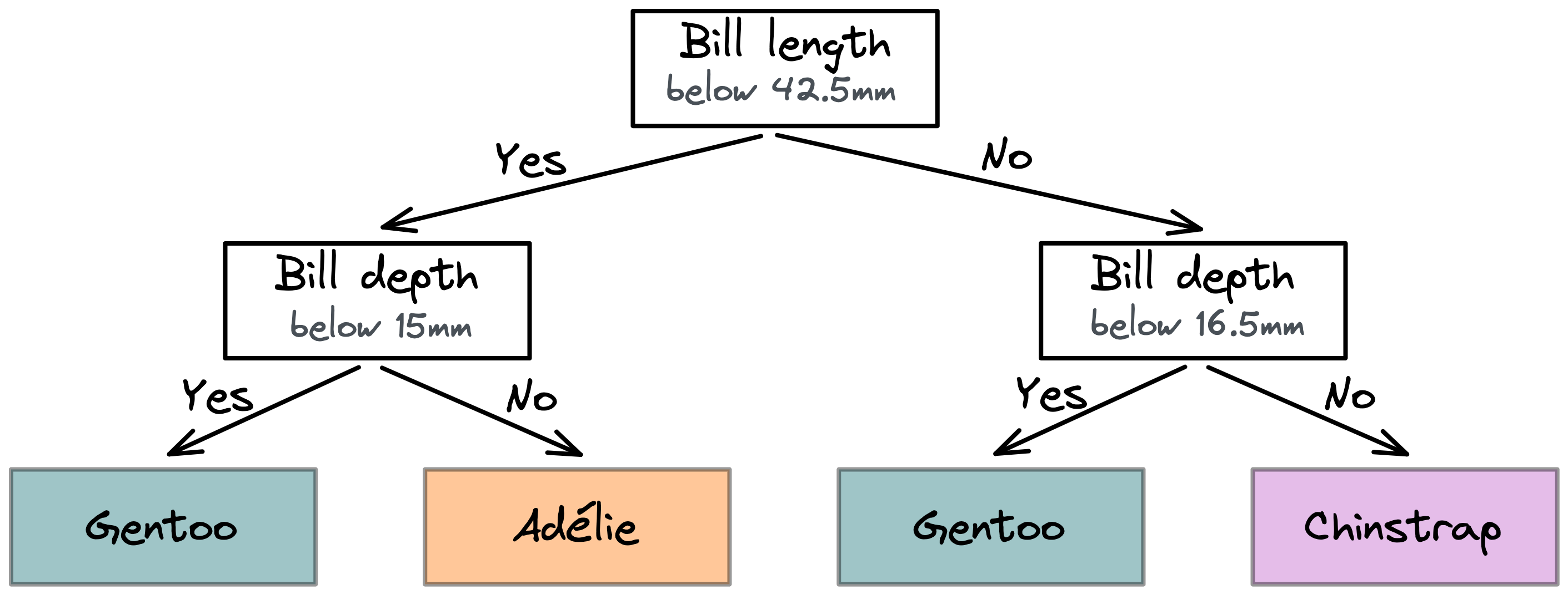
This is exactly what a decision tree model does: it identifies suitable decisions that split the data into separate regions. It tries to do so to optimally associate each region with one particular class. In our example, the model made two consecutive decisions that resulted in two rounds of splitting the data.
If we visualize these splits on the previous graph and highlight which regions belong to which species, we would get the following figure:
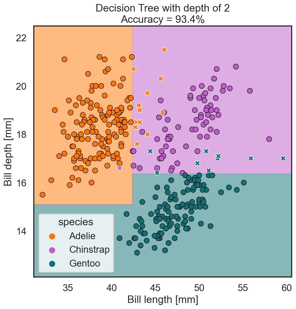
What we can see here is that the decision tree model with two rounds of splits is capable of separating the three species with an accuracy of 93.4%. Meaning it still makes a mistake in 6.6% of the observations, which are shown in the plot as x.
Now let’s see what happens if we allow the AI to do four, six or eight rounds of splits:
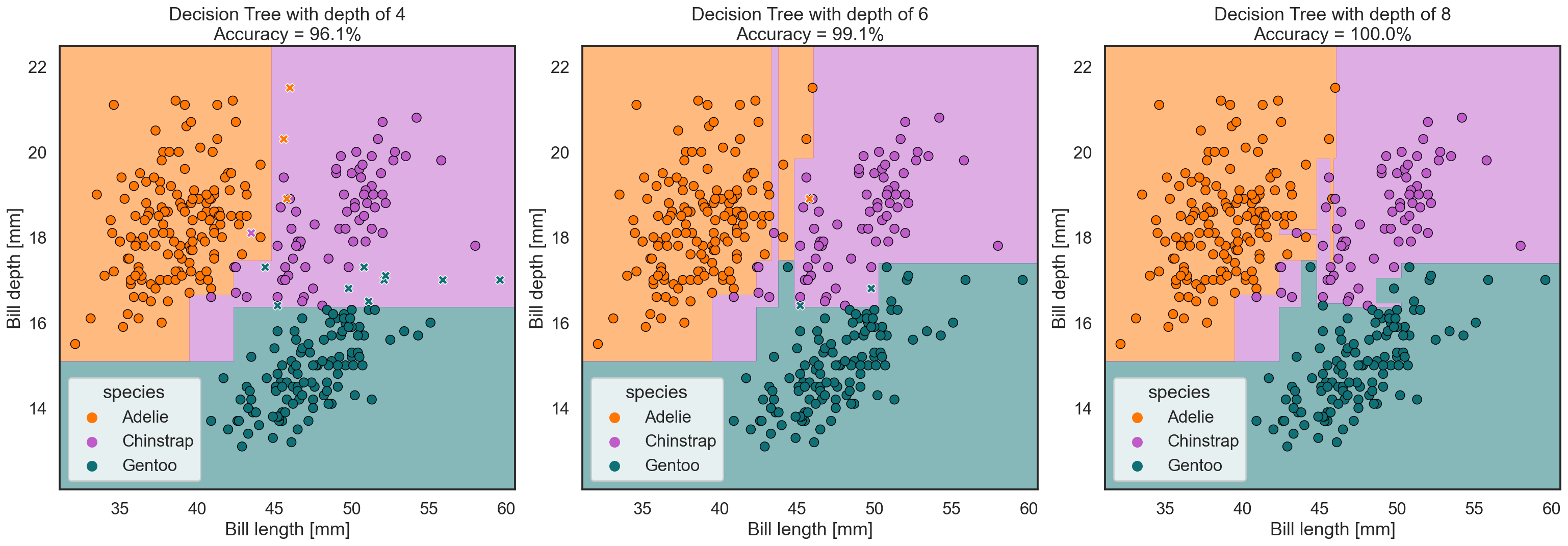
What we can observe is that the region belonging to a species becomes more characteristic the more rounds of splits we allow. And at the same time, the classification accuracy goes closer to 100% until the model doesn’t make any mistakes anymore.
But as we mentioned before, some mistakes may be acceptable if in return we avoid creating very unnatural looking class regions. Such jagged and unnatural regions would work well for the data we have recorded up to now and with which we trained our model, but they might not work that well for new data points we may record in the future. Therefore a decision tree with four levels of splits might ultimately represent and predict the reality we live in better – it works well for the current dataset, but it is also flexible enough (i.e. not too opinionated) to handle new recordings in the future.
In the context of machine learning, figuring out where to split the features (e.g. bill depth at 42.5mm) is what we call model training. The AI uses the data to identify the most optimal splits, hence different data can lead to slightly different models. And figuring out the optimal amount of rounds of splits is what we call learning. The AI would learn that four rounds of splits is most optimal for the current dataset, but also for all potential future recordings. Or in other words, the AI learned that a model parameter of four leads to the optimal model performance on this dataset.
K-nearest neighbors – the finding similar observations approach
Let’s now explore how another classifier model would solve the penguin problem. For this, we will examine the k-nearest neighbor classifier. As the name implies, this model looks at the nearest observations (i.e. neighbors) to identify the class of a new data point.
For example, let’s imagine we have a dataset with points on the left belonging to the class ‘purple’, while points on the right belong to the class ‘green’. Now, to which class would you assign a new observation ‘x’ – purple or green?
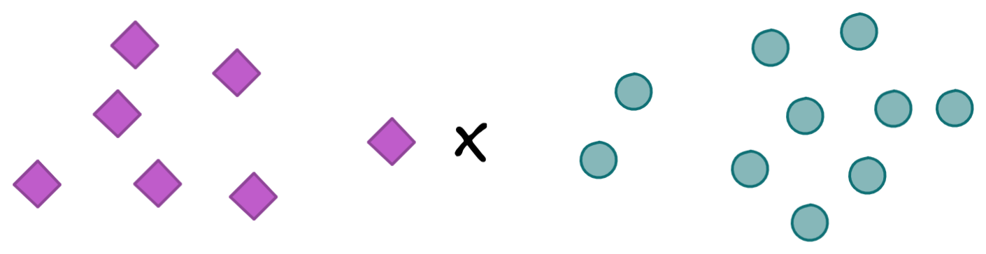
Well, if you use a k-nearest neighbor approach, the decision would go as follows:
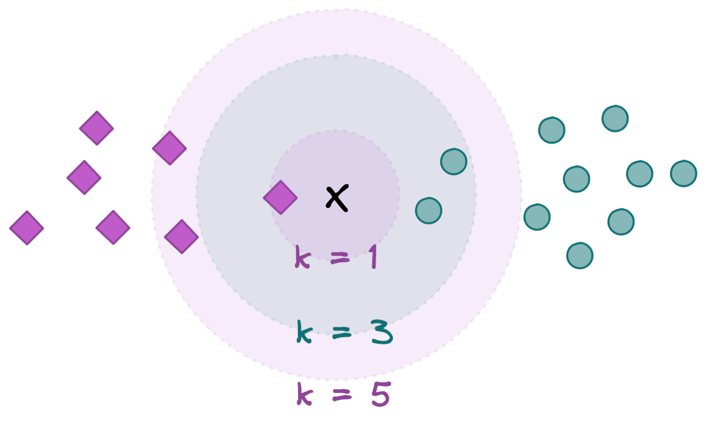
- K=1: Looking at the closest one neighbor, which is purple, we would assume that the new observation ‘x’ belongs to the class purple as well.
- K=3: Looking at the closest three neighbors, of which two are green and one is purple, we would assume that the new observation ‘x’ belongs to the class green, as this colour is more likely.
- K=5: Looking at the closest five neighbors, of which three are purple and two are green, we would assume that the new observation ‘x’ belongs to the class purple, as this color is more likely.
K-nearest neighbor models have the great advantage that they are rather simple to create; no complex mathematical equations need to be solved. However, to find out which five points are the closest to a new observation, we first need to calculate the distance of the new observation to every other datapoint in the dataset, and that can become very time consuming. Depending on the size of the dataset, computing the distances between all points either takes a very long time, or might not even be possible.
Now let’s see how such a nearest neighbor model would perform the penguin species classification task:
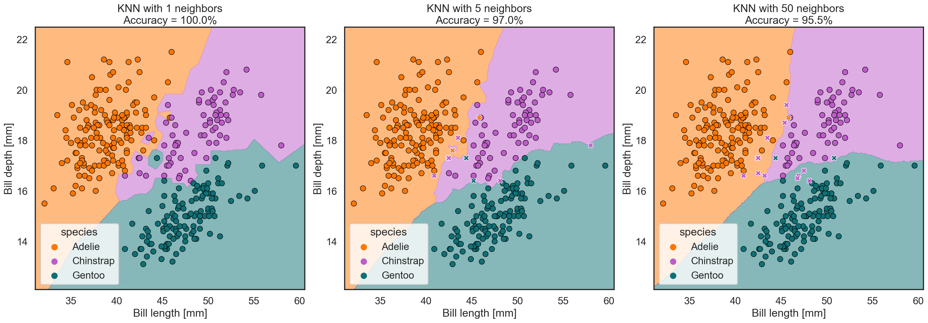
If we choose k=1, our model will always achieve 100% accuracy for this dataset. Which, as we saw before, might actually be a bad thing. This model creates class regions that look like small islands, around every point. Such a model is too focused on the dataset it was trained on and will fail to correctly predict the class of new specimens.
With k=5, we already make a few mistakes, but the class regions still look very unnatural. With k=50, the outlines are becoming much smoother. While this model ‘only’ reaches an accuracy of 95.5%, the regions look much more like what we humans would potentially draw.
In this case, a higher k is better than a lower one, but this doesn’t need to be the case for other datasets. Just as before, finding the right model parameter (in this case the right k parameter) for the task is what we call learning – the AI learns the most optimal value k for the recorded dataset, and for new penguins we might measure in the future.
Support vector machine – the identifying representative samples approach
Yet another type of machine learning model that can be used for classification is the support vector machine (SVM). To better explain what this kind of model does, let’s consider the following figure with two clusters of purple and green dots.
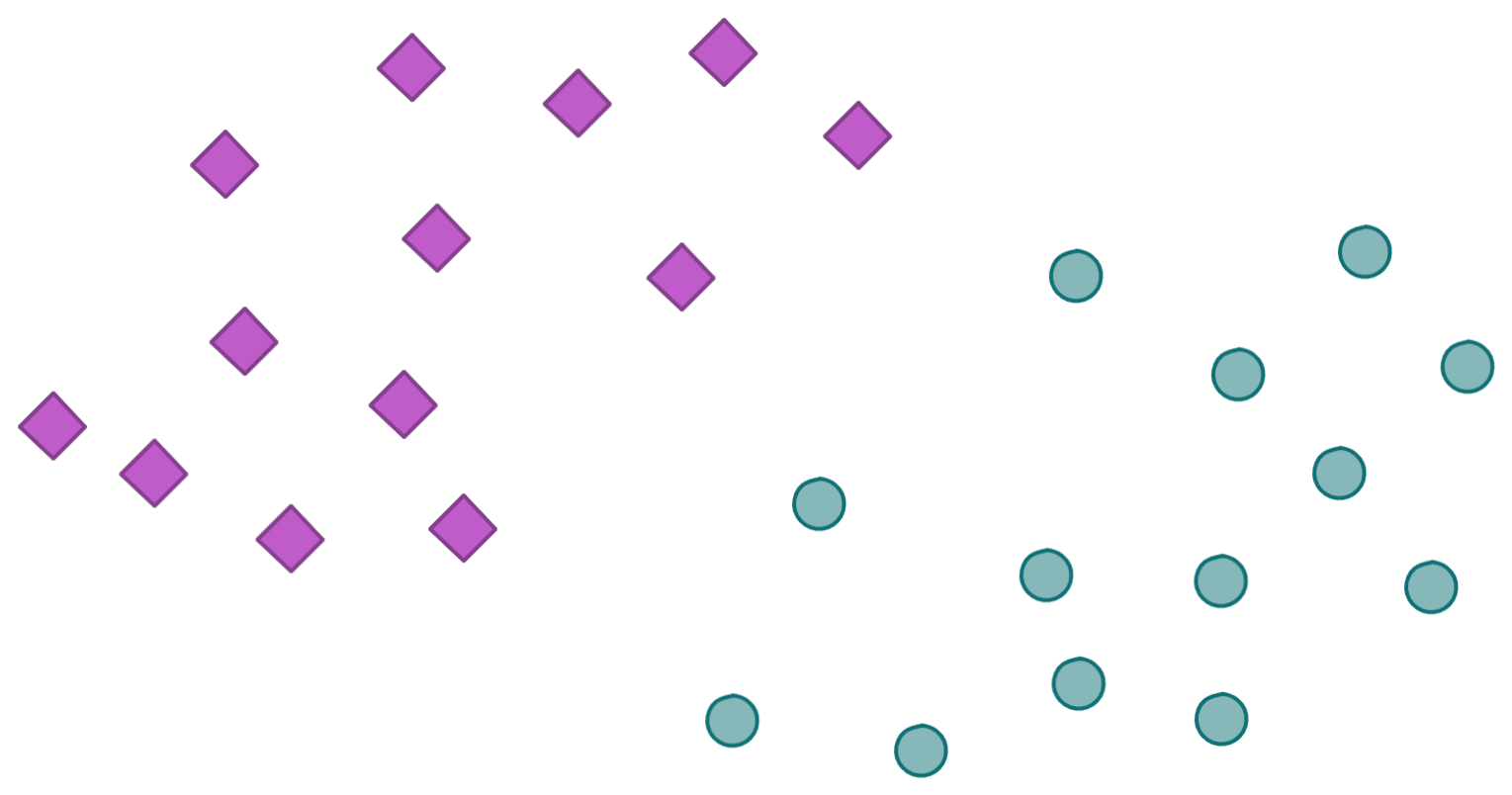
As we’ve already seen in the other models, the goal of a classifier is to identify which regions of the dataset belong to one or the other class. In other words, the goal is to find a border line that would separate these two classes from each other.
Support vector machines (SVM) do this in a very elegant way. By examining the data, the support vector machine tries to identify ‘representative’ data points at the border between the colored clusters that can help to separate these classes. In the next figures, these points are annotated with a black dot:
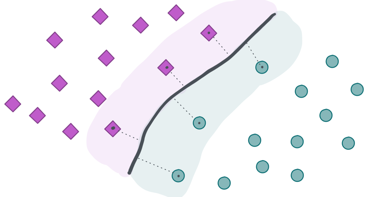
The data points that are closest to the border (the ones with the black dot) are called support vectors. This is because they are supporting the definition of this border. Furthermore, for each model we can also specify how far the reach of these support vectors should be and how many mistakes are allowed on the wrong side of the separation line. In other words, should only a small region around a support vector be colored in green or purple, or should it do that for a wider region, allowing for some mistakes?
We can see why these things are important by coming back to our penguin dataset. Let’s take a look at how a support vector machine would carry out the task of identifying our three penguin species:
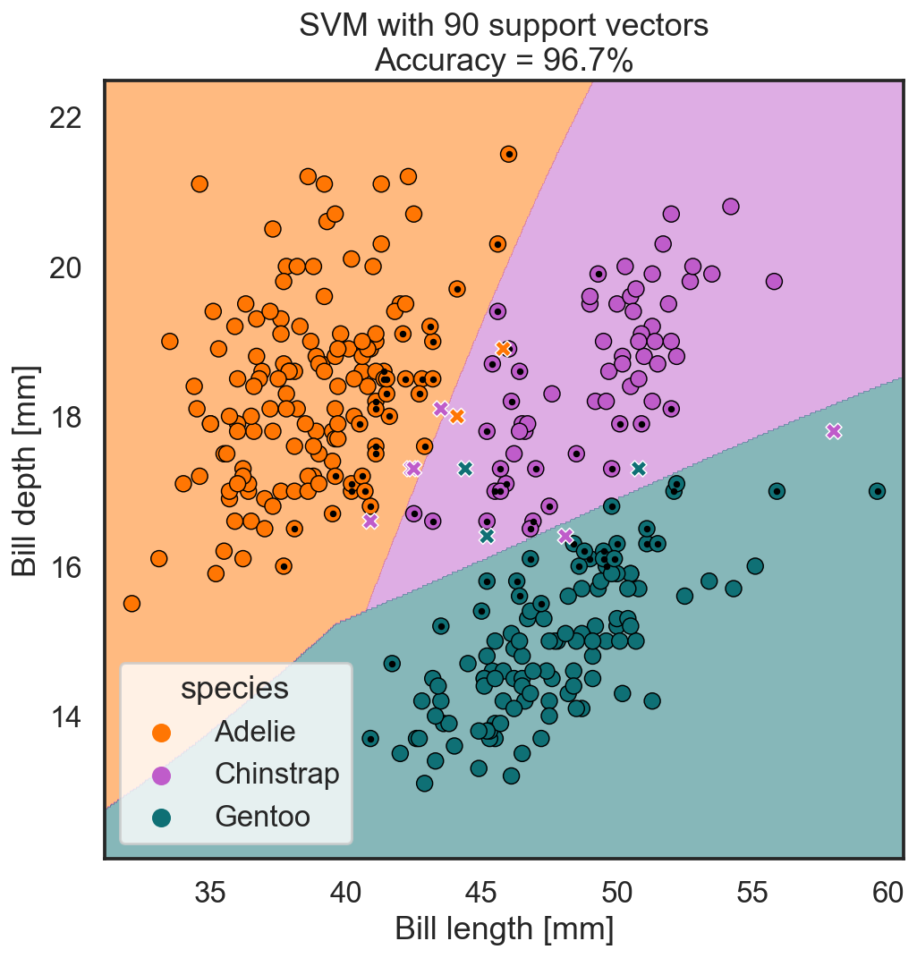
By using 90 support vectors, our model reaches a classification accuracy of 96.7%. That figure seems to be well separated into the three species, more or less how we humans might do it.
In the following figures you can see what happens if we ask the model to use a lot of support vectors with very small margins (left), or only very little support vectors with wide margins (right):

In both cases, our models reach classification accuracies of 99.7% – much better than we achieved before. However, we can easily see this solution is again less effective than the previous approach. While the coloring of the regions for the three species seems to work for our current dataset, it seems unlikely that it would work for newly measured penguins.
Once more, the model uses the data to identify suitable support vectors. By trying out different numbers of support vectors and different sizes of margins, the AI can learn what the best combination might be.
Summary
In this article we have learned about classification and saw that a machine tries to solve this task in a comparable way to us humans. And just as there are multiple strategies to how we would solve this task, there are also numerous ones for the machine.
- In decision trees, the machine learns the optimal number of splits it should perform and at which values.
- In k-nearest neighbor models, the machine learns the optimal number of neighbors to consider.
- In support vector machines, the machine learns the optimal number of support vectors and how much margin around these points it should use.
These are just a few machine learning models that can be used for classification, and there are many more. But what all of these approaches have in common is that the AI tries to learn the optimal model parameters to do the classification task well enough to be useful, but still with some mistakes to ensure that the learned regions are also useful for future measurements.