Artificial Neural Networks

When you think about it, many of humankind’s great inventions and breakthroughs were triggered by stories and legends.

The legend of Icarus pushed us to invent the plane, while submarines and underwater diving were mentioned in the legends of Alexander the Great; it would be difficult to imagine flying in the sky or diving under the water for a long time if we had never seen birds or fish. Jet packs appeared in science fiction stories as far back as the 1920s, automatic doors featured in Herbert Wells’ books, and tablets in Stanley Kubrick’s movies. Today, we have the ambition to create an AI – an artificial intelligence – that is on a par with our own human intelligence. An artificial or digital brain inside a computer, so to speak.

From imitation to understanding

Our first naive attempts at AI (at least in literature) were copying the concept as is: Icarus built his wings from feathers and wax, and Frankenstein tried to build an artificial human from the parts of other humans.

However, at some point it became clear we have to transfer the concept, rather than blindly copying nature. The creation of planes supports this claim. To build a plane’s wing we used the same principle as the bird’s wing, but rather than focusing on the fact that a bird’s wing is full of feathers, we realized that it’s the shape that creates lift and keeps the animal in the air.

The same is happening with our attempts to replicate human capabilities by creating artificial intelligence. Once we began to understand how the human brain works, we started replicating it – and by that we do not mean building a physical copy of it, but rather trying to mimic the principles of what the brain does. Our understanding of how the brain works triggered a whole new area in AI, called ‘artificial neural networks’.

The mechanics of the human brain

The human brain is an extremely complex system, which is not fully understood – yet. However, there are several things we already know. For instance, the brain is built from hundreds of billions of specialized cells called neurons. These cells are interconnected to each other in a fast biological network, allowing one neuron to send its signal to many other neurons. In this way, information can be passed from one part of the brain to another by transmitting signals through these connections.

For instance, when we see a speed limit sign, one part of the brain analyzes what’s displayed on the sign. This message is then transmitted to the part of the brain which decides what to do next (e.g. slowing down). This intention is then passed further on to the motor centre in the brain that controls the muscles in your foot and initiates the actual braking.

But that’s not all. By passing a signal from one part of the brain to another, the information carried through the network may change from place to place. In our previous example, the first signal that enters the brain is the visual information from the speed limit sign, which is then transformed into the information that we should slow down, which in turn gets transformed into the information of moving the muscles in the foot.

A typical neuron performs three distinct actions. First, it receives and collects information from one or multiple neurons that it is connected to. Second, it processes all of these inputs and decides if the overall information is important enough to pass on further. And third, if it decides to pass the information further, it will send it to all the neurons it is connected to. However, it might decide to slightly change the signal – making it either stronger or weaker – depending on how important that neuron finds the information.

A simple learning network

Remember your first high school class? Let’s consider this class as a network, where your classmates and you are connected. You get a message from a couple of your friends that the class is dismissed and they decide to go for a walk instead. At this point, you have to decide whether it is true information and a good idea to pass it further – or if it is simply a trick to skip the lesson that you shouldn’t tell your other classmates.

But how do these neurons help the brain to work? As it turns out, once you connect millions upon millions of such neurons into a huge network, some of these neurons can become very specialized.

Imagine a baby that has only ever seen a couple of rabbits in their short lifetime. If the baby sees a new animal, how can it tell if it’s a rabbit? The baby will probably look for the features of rabbits that it has seen before, such as long ears, a fluffy short tail, and long hind legs. If the baby then sees an animal in the zoo that has long ears, a fluffy short tail, and long hind legs, then they would know it is a rabbit.

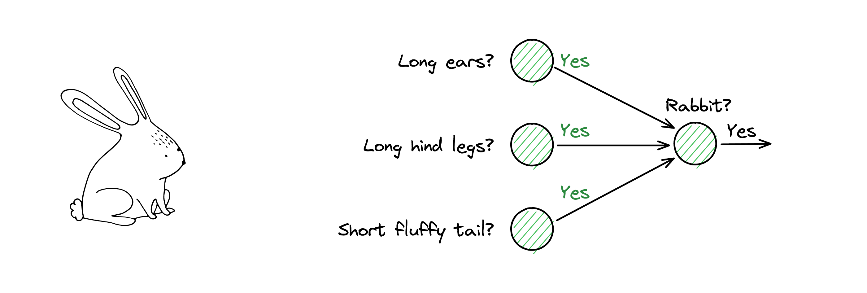
Easy, right? It’s equally simple to think about it in terms of neurons. Imagine we have three neurons that are able to detect if an animal has long ears, a fluffy short tail, or long hind legs. Each of these neurons pass the message further to the next neuron, only if it detects the respective feature (i.e. the “long ears” neuron will send the message if it sees long ears). The next neuron in our chain identifies a rabbit, only if it collects enough messages (let’s say all three messages). If it collects less than three messages, then the neuron can’t be sure it’s a rabbit.

For instance, a kangaroo has long ears, long hind legs, but no fluffy cute tail. If our final neuron receives only two messages from “long ears” and “long hind legs”, it cannot confidently identify a rabbit. In other words, such a “rabbit detection neuron” needs to receive three messages as input for it to become active. If the signal doesn’t reach this threshold, the “rabbit detection neuron” will remain inactive.

Artificial neural networks

Due to its enormous number of neurons, it’s extremely difficult to recreate an exact copy of the human brain. Ultimately, that’s not our goal – we need to move from the bird’s wing to the plane’s wing and translate our simplified plain English description of how neurons work to the language that a computer would understand.

To achieve this, some math is required. However, you won’t see anything more complicated than adding or multiplying two numbers, and identifying whether the number is greater or lower than zero. With these three simple operations we are able to build an artificial neuron that mimics the mechanism of a biological neuron.

Let’s also consider the messages as numbers. For simplicity, instead of applying the abstract term “long ears”, we’ll let this neuron return the length of ears in centimeters. The same applies to the “long hind legs” and “fluffy short tail” neurons, which would also be measured in centimeters.

We also need to figure out how the neuron would collect these numbers from the other neurons connected to it; we will call these numbers input connections. The simplest approach with this bunch of numbers is to sum them up. Coming back to our example, the final neuron takes the inputs from the previous neurons (“long ears”, “long hind legs”, “fluffy short tail”) and adds these numbers together.

For now, the three feature numbers – standing for “length of ears”, “length of hind legs” and “length of tail” – each have the same importance. That is, receiving 30cm from the “length of ears” neuron would have the same meaning as receiving 30cm from the “length of legs” neuron (cats, for instance, might have similar length legs). The problem is that having long hind legs is not as important as having long ears (have you ever seen a cat with 30cm long ears?).

We could tweak these feature numbers by multiplying them by other numbers, which would represent the measure of importance, and thus increase or decrease the contribution of each feature number to the total. For instance, to have a weaker importance, the “length of legs” connection is multiplied by 0.1 (yielding 3), while the more important “length of ears” connection is multiplied by 1.5 (yielding 45).

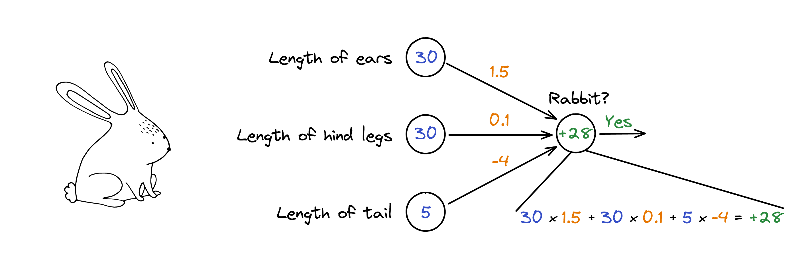
Note the relationship: the longer the ears and legs, the more rabbit-like the animal. This relationship does not hold for the tail. In fact, it is inverted: the longer the tail, the less rabbit-like the animal (think of the kangaroo).

Let’s say we will need to multiply the length of the tail (5cm) by -4, which will yield -20. These measures of importance are unique for each neuron, and we will call them weights.¹ We’ve encountered such ‘measures of importance’ already before in the article A peek behind the curtain, where they were referred to as ‘parameters’. While ‘weights’ and ‘parameters’ represent the same thing, people usually use the former when talking about a neural network model and the latter when referring to a more classical machine learning model.

Now that the neuron has collected the input signals, it needs to decide whether it is a rabbit and, if it should become active, send the message further (the output of the neuron). So, how can we decide if it is a rabbit or not?

Imagine that we have a kangaroo instead of a rabbit. In this case, the neuron should tell us this is not a rabbit (and thus not to send the message further). Let’s say the kangaroo has the following measurements: length of ears 30cm, length of hind legs 50cm, and the length of the tail 50cm. Keeping the same weights, our neuron would output -150. Since we do not want to send a message further because it is a kangaroo, we introduce a very simple rule: if the sum is below zero (negative), we won’t send the message further – otherwise we will send a message further. The content of the message will be that sum; think of it as a filter where only positive messages go through.

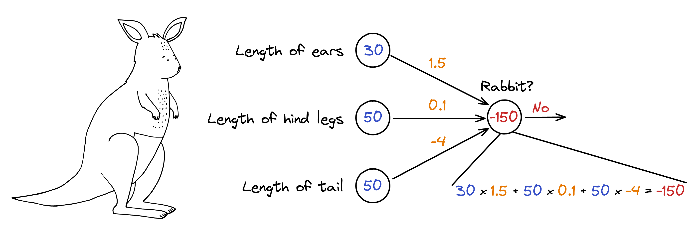
For this Australian marsupial, the sum is -150. As this is below 0, the neuron won’t send the message further (and because it’s not a rabbit).

Are you ready for a small stretch for your own non-artificial brain?

What would be the final neuron output of the image below? You can find the solution in this ².

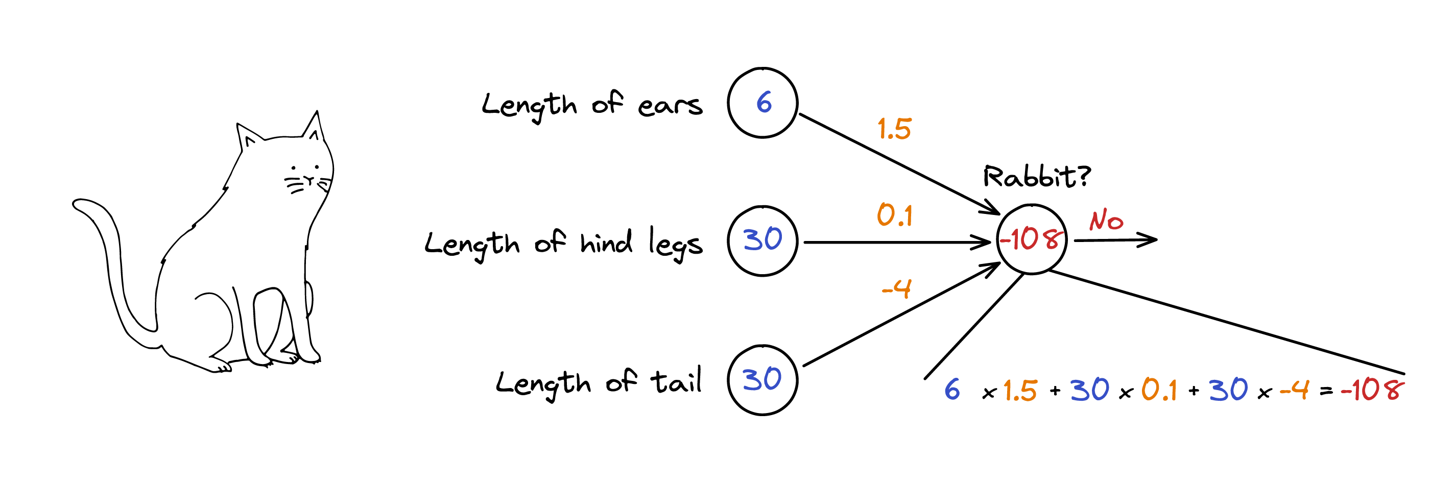
And this is how we pass messages in the form of feature numbers from the left as inputs through the network, to the right and receive an output. This passing through is also called “forward propagation”, because we move forward through the network.

And that’s it! This simplified representation of a neuron was a turning point in the world of AI. As Neil Armstrong would probably say: “That’s one small step for a neuron, one giant leap for the network.”

How the learning process works

When considering the rabbit example, there is something else to consider. How do we get the values of those weights (i.e. those numbers in red)? To answer this question, we need to zoom out and see the global picture of the artificial neural network’s purpose – the unique way it learns from what it ‘sees’.

To understand the phenomenon of learning, we should go no further than your favorite pizzeria. If you are a regular customer who orders the same thing every time, Bob the waiter will greet you with the phrase, “Same as usual?” No wonder, Bob has seen you ordering the same pizza so many times, he simply memorized that you always order a diavola.

But let’s dive deeper. Somehow, Bob can guess what kind of pizza a customer will order by only looking at them. For instance, if a customer is from Sicily, Italy, they will probably not order a Hawaiian pizza. Or if a customer seems to be very ecologically conscious, then they will likely go for a vegetarian one. How has Bob developed this sense for customers’ pizza preference?

The secret is in the way our brain learns the information. Bob has seen numerous customers and implicitly learned the rule of how to associate the pizza type with the person’s appearance. With each new customer, Bob firstly sees an appearance, then tries to figure out what kind of pizza will be ordered. If he makes a mistake, his brain readjusts the rule, so that when he sees a similar person next time, he makes a correct guess.

Projecting this example onto the artificial neural networks, Bob learns the weights of a neuron by observing a huge number of instances (i.e. customers). By making errors, he tweaks the weights of the neurons in such a way that he can predict the type of pizza correctly the next time. In other words, Bob tries to minimize the chances of guessing the wrong pizza.

The giant leap

From the mathematical point of view, what Bob’s brain performs (tweaking weights to get a more accurate model) does not look to be a complicated problem if we use several neurons. For instance, the grandfather of modern networks, the perceptron³ (developed in the late 1950s) could handle this task. The perceptron is a very simple artificial neural network, just like the networks that we have seen so far (e.g. the “rabbit” network). Given the sizes of legs, ears, and a tail, the perceptron could identify a rabbit.

However, there was an issue with the perceptron: there were relatively simple relationships between the input and the output that the perceptron could not represent. Probably the most famous one is the so-called XOR relationship, also known as the exclusive or. In short, it depicts the relationship that something is true if (and only if) condition A OR condition B is true – but not if A AND B are true.

For example, let’s look at the following four statements:

“If it is night outside, and it does NOT rain -> True, I will go outside” “If it is NOT night outside, and it does rain -> True, I will go outside” “If it is night outside, and it does rain -> False, I will NOT go outside” “If it is NOT night outside, and it does NOT rain -> False, I will NOT go outside”

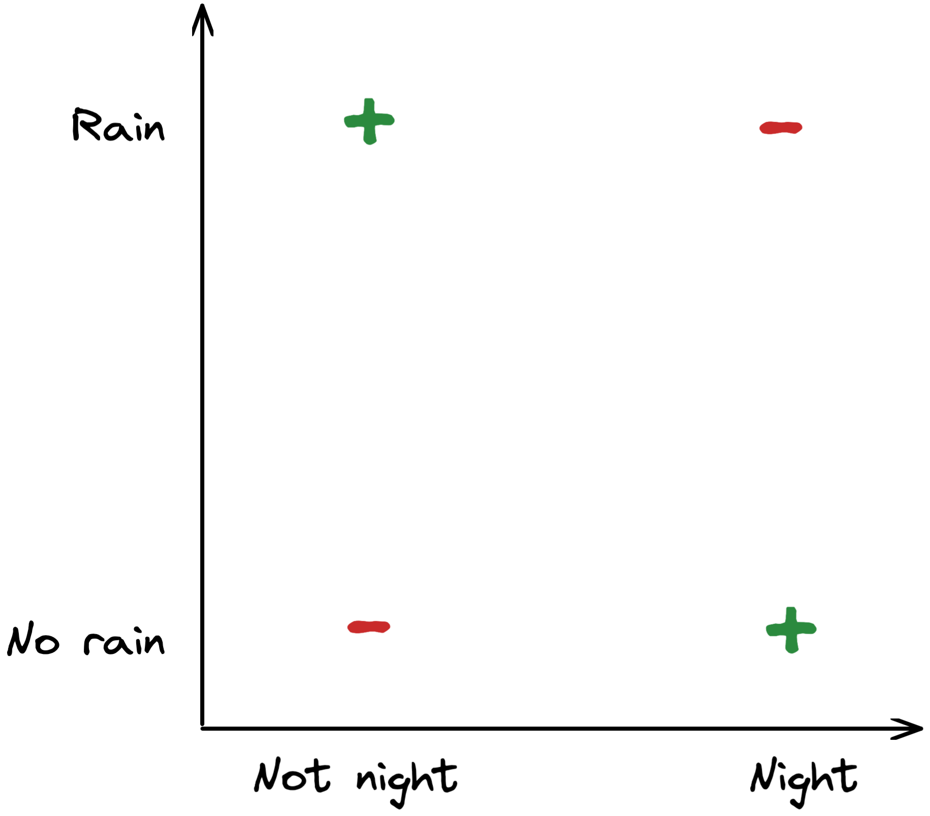
Such a particular XOR relationship cannot be implemented in one single perceptron. No combinations of weights allow the following perceptron to give the right answer to all four statements above.

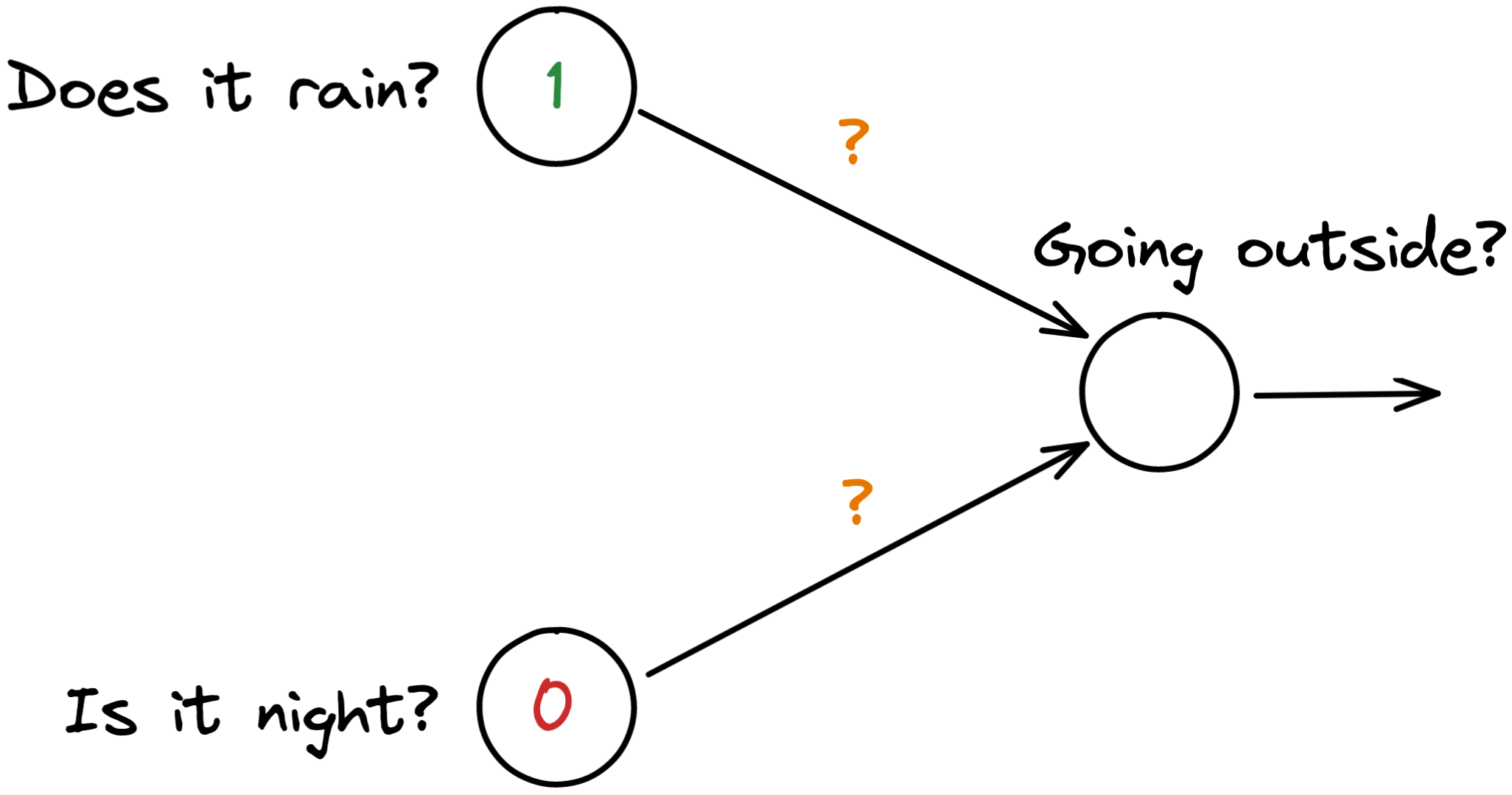
However, by adding a few more intermediate neurons in the middle of the network, our artificial neural network can start to learn more complex relationships than previously possible. As these intermediate neurons are neither part of the input nor the output neurons, they are also called ‘hidden neurons’. Thanks to these hidden neurons, a neural network is capable of capturing intricate information patterns and is able to represent things like the XOR relationship – and much, much more.

While these additional neurons allowed us to capture complex patterns, the advantage gained came at a price: our old way to train these models, the one used for perceptron, did not work anymore. It was too simplistic. And so we had to invent new and efficient algorithms that would allow such a network to learn. It took almost 30 years before we figured out the backpropagation algorithm,⁴ which allowed us to train networks with hidden neurons. The invention of this algorithm was an actual “giant leap”, which Neil Armstrong would be very proud of.

The power comes from layers

In the previous section we introduced hidden neurons, but we didn’t discuss the way they are organized. Here, we again took inspiration from the human brain, where the neurons are organized in layers.

The illustration below shows two ways to organize the network with the same number of hidden neurons. For example, we can place all 10 hidden neurons in one row, or we can make two rows of five neurons.

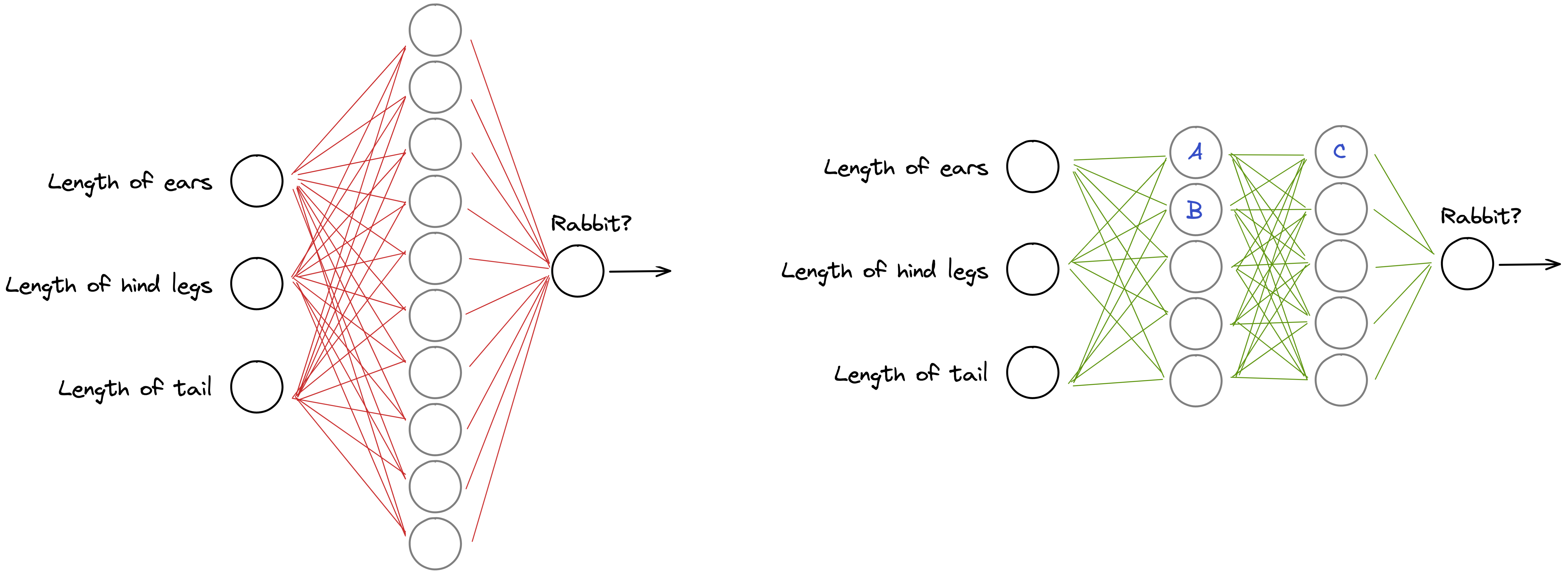
The second architecture works better than the first one for two key reasons. Firstly, the second architecture has more connections (45 green lines versus 40 red lines) and therefore can learn more unique relationships. It may not sound like a lot, but for a larger number of hidden neurons, these differences are significant. Without going too deep into the specifics, more connections or weights on multiple layers means a more flexible model that can look for a wider range of information patterns.

The second reason is less intuitive, but perhaps more important. The architecture with two layers allows for the capture of the interdependence between the nodes of the previous layers. It could be mind-boggling to explain this in terms of the numbers, but the interpretation is relatively simple.

The higher layers (the ones closer to the output of the “rabbit” neuron) capture higher-level patterns. For example, neuron A can look at the relationship between the long hind legs and the short tail (let’s call it the rear body part neuron). Then neuron B is responsible only for the long ears (the front body part neuron). The interaction between these neurons is captured by neuron C (the full body neuron), which is then passed to the output neuron. Neuron C looks at the higher-level pattern (full body), and neurons A and B consider lower-level patterns (the rear and the front body parts). Imagine these patterns are organized hierarchically, and the layers closer to the output layer are triggered by higher-level patterns.

It’s because of the automatic detection of such high and low-level patterns that artificial neural networks are so powerful. Previously, researchers had to manually create tools to extract meaningful patterns from a dataset. And by doing so they had to judge ‘should we look for ears or legs – or both?’. Now the neural networks can complete this task by itself; there is no need for manual intervention or guidance. If a neural network thinks it’s most useful to look for colours in an image, or for fluffy ears, it will do so. Similarly, if it needs to look for eyes, ears, and a nose in an image to detect a face, it adopts that process. If the data shows it, the neural network can learn it.

These patterns are not always easily interpretable, and normally we do not know which pattern triggers one or the other neurons. That is why you might hear some people refer to neural networks as black boxes. Intuitively, the more layers we have, the finer the hierarchy of patterns that can be considered by the layers.

However, as with so many things in life, too much can also become an issue. Generally speaking, the more layers we have, the more complex relationships we can capture – but only if we also have enough data to train the model and learn all of these millions and billions of weights.

Deep neural networks

In this article, we’ve already learned multiple important concepts: an individual artificial neuron receives multiple inputs, sums them all together, and based on a threshold, decides if this information needs to be given further. And when you connect multiples of these neurons together in layers, you create an artificial neural network.

In this case, the first layer of the neural network (where the input comes in) is conveniently called the input layer, while the last layer (where the output goes out) is called the output layer. It’s this last output layer that tells us that an image contains a ‘rabbit’ or that tomorrow’s weather will be ‘sunny’ with a 30% chance of rain.

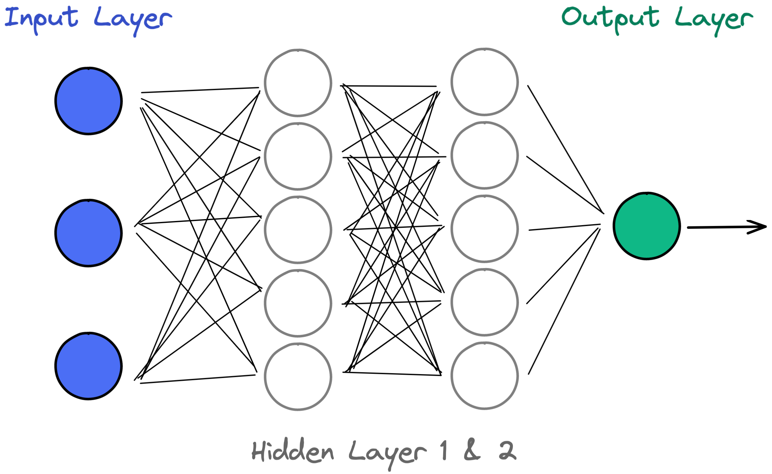
All other layers of neurons between the input and output layers are called hidden layers. They are “hidden” because it is much more difficult to say what these individual neurons actually do. They receive input and create outputs which can often only be interpreted by the machine. The number of hidden layers varies throughout the years. In 1990, several hidden layers were considered groundbreaking. Nowadays, the number of hidden layers can reach several hundred.

We say that an artificial neural network with at least one hidden layer has some ‘depth’ to its architecture – which is the reason why we also call them deep neural networks. Therefore, because of this characteristic, training such deep neural networks is fittingly called deep learning. We will go into more details about deep learning in a future article.

Deep neural networks were a big game changer in AI research for many reasons. Having multiple hidden layers allows a network to identify intricate patterns in the dataset, learn non-linear or non-obvious feature relationships, and all without the need of a human in the loop. Once the network architecture is set up, the only thing missing is appropriate data, and backpropagation does the rest.

Furthermore, the computational demand for each individual training step is often minimal, and so neural networks scale very well with data size and can easily analyze huge amounts of data (also known as big data). And thanks to the complex interconnections between neurons, a deep neural network can analyze the input data in multiple ways and identify numerous important patterns, all at the same time.

Thanks to these powers, deep neural networks are able to identify objects or people in a picture, drive cars for us, understand spoken words, and translate text into more than 100 languages at once. Every year, researchers come up with more advanced network structures, which allows them to solve evermore fascinating tasks. We will cover many of these different network types and what they can do in later articles.