Dimensionality reduction describes the process of identifying lower-dimensional structures in higher-dimensional space – or in other words, when we try to make ‘big data’ smaller and more compact so that we humans can better understand what’s in the data, and our computers have less of an issue of handling it.
Dimensionality reduction describes the circumstance where we summarize a multitude of different characteristics about something (i.e. dimensions of information) into a few but meaningful descriptive characteristics.
For example, let’s imagine you travel from Zurich to Tokyo, a 12-hour direct flight. The person next to you is very talkative and you learn all about them: they love to travel by plane, train, car and bike, but not by boat; they love to run, hike, climb and paraglide, but hate swimming; they love dogs, cats, birds and bears, but not fish. Each piece of information is another dimension of who they are and is what makes them unique.
So let’s summarize what we just learned about this person:
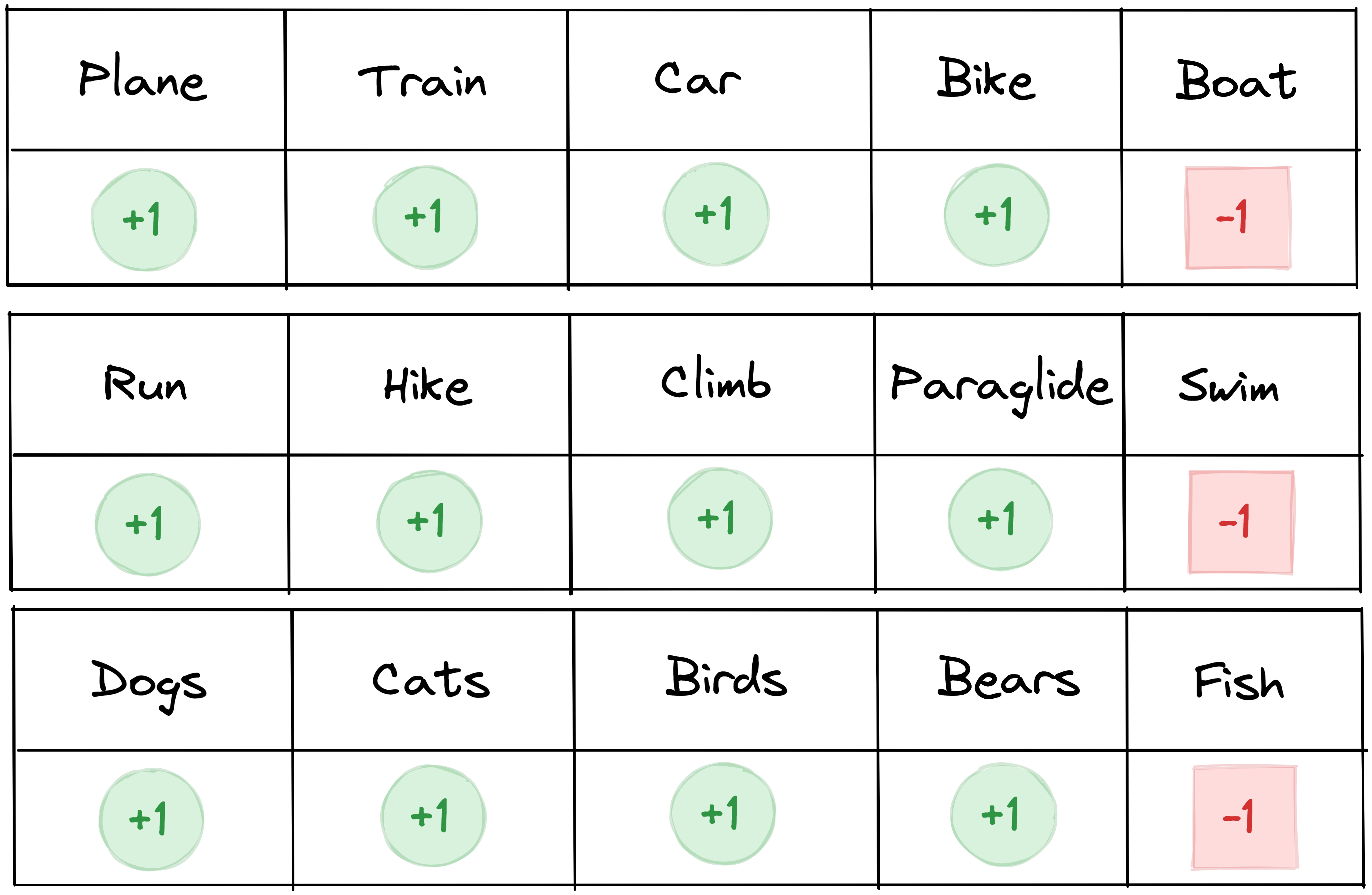
What we have tabled is this person’s preference for 15 different things. In the context of machine learning, we could also say that this person can be represented as a single point in a 15-dimensional space. If you yourself have the exact same preferences, then your point would be at exactly the same location in this 15-dimensional – or high-dimensional – space.
What dimensionality reduction allows you to do is reduce this information to fewer dimensions than the original 15. For example, the positive preferences (highlighted in green) could be summarized into three dimensions: ‘loves to travel’, ‘loves to do sports’ and ‘loves animals’. Meanwhile, the negative preferences (highlighted in red) could be summarized into one additional dimension: ‘doesn’t like any activities or things connected to water’.
So from 15 dimensions, we were able to reduce this person’s preference to four more meaningful characteristics. Or in other words, we reduced the dimensionality of this dataset from 15 to four – from high-dimension to low-dimension.
Finding out which features to combine in what way – and how to reduce the dimensionality of the data while still keeping as much of the original information as possible – is the interesting and challenging domain of dimensionality reduction.
Machine-based dimensionality reduction
In a previous article, we learned that the task of dimensionality reduction belongs to the machine learning category of unsupervised learning. In unsupervised learning, we try to find useful structure in our dataset that we hope to exploit later on. However, in contrast to supervised learning, in unsupervised learning we don’t have a target label to guide us during our approach.
An AI that performs dimensionality reduction tries to transform the original dataset into a different representation where the dimensions are more useful to learn from, or where they are easier to understand for humans.
Artificial intelligence performing dimensionality reduction can be encountered in multiple settings. For example:
- Meaningful data compression: Reducing a dataset from high to low-dimensions also means that you reduce the volume of the dataset on your hard drive. In computer terms, this can also be called data compression. Just like JPEG images are a compression of other image formats, the aim is for compression to keep most of the relevant information in the data intact, so that objects are still well enough represented.
- Noise reduction: A neat side effect of dimensionality reduction is that the removed dimensions often represent unnecessary details in the data which can be removed without losing any relevant general information in the dataset, because only the noise is eliminated. This approach can be used to remove noise from images and audio recordings, or to clean out noisy sensory signals coming from other machines.
- Data visualization: We live in a three-dimensional world, which means that we can only visualize data in one, two or three dimensions. Anything of higher-dimension cannot be visualized on paper or in our mind. Dimensionality reduction can offer a solution to this shortfall when working with multi-dimensional datasets. By reducing any high-dimensional dataset to just two or three dimensions, we can potentially visualize important structures in the data, gain new insights, and perhaps even identify clusters. This is a very common approach when working with big data.
How humans perform dimensionality reduction
At first glance, humans are not very good at dimensionality reduction. Let’s imagine somebody gives you a list of 40 characteristics about a person and you are asked to reduce these to a few key features. It might take five minutes, but you should be able to do it.
But what about 400 characteristics? How about 4000? What if you knew a person’s preference for every single food item, animal, sport, hobby…? There’s just not enough time to reasonably look at all of this information.
Luckily for us, as a species we came up with a strategy of performing dimensionality reduction – at least in the context of describing things – with our language and the creation of new words.
For example, instead of saying that you have muscle weakness, poor concentration, slowed reflexes and a slow response time, you could also just say that you’re exhausted. Similarly, being vegan provides a lot of information about your eating preferences without going into details about every individual food item.
Thanks to our language, we can communicate a lot of information with only a few words. To put it another way, we are able to communicate a high-dimensional dataset in just a few words (i.e. as a low-dimensional dataset).
How machines perform dimensionality reduction
The goal of dimensionality reduction is to change the representation of a dataset in such a way that it preserves the relevant qualities of the original data. Different dimensionality reduction approaches measure these relevant qualities in different ways. To get a better understanding of how an AI can learn to do this task, let’s explore three different approaches: projection, manifolds and autoencoders.
The goal of this exploration is not to teach you the intricate details of these three approaches, but to show you in a hopefully intuitive way that there are many different ways a machine can go about reducing the dimensionality of a dataset.
Projection
In the context of machine learning, a projection is a mapping of points from a high-dimension down to a lower-dimension, where the direction of the mapping is exactly the same for all points.
Similarly, when you are at the cinema and by chance stand in front of the movie projector, the image of your three-dimensional body will be projected onto the screen as a two-dimensional shadow. Even though the depth information might be gone, everybody can still recognize that it’s you.
To better illustrate how projection works, let’s take a look at the following point cloud in a three-dimensional space. While we can clearly see a structure in this dataset, namely a circle, it is difficult to describe this circle simply in terms of x, y and z.
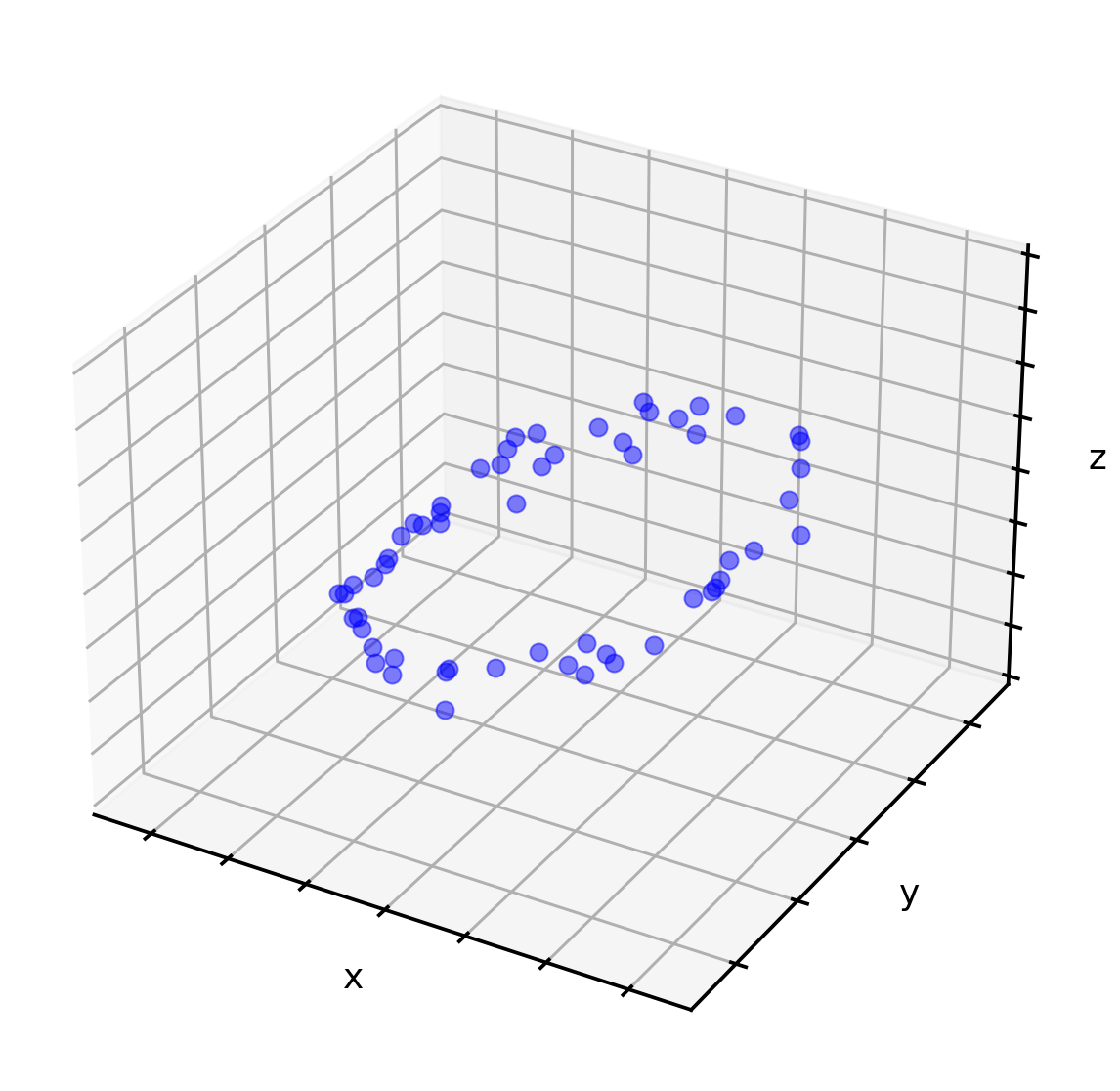
However, we can identify a plane that can be put through the point cloud so that the projection of these points onto the plane still shows the relevant shape of the circle. In the following illustration, this plane is visualized in green. The red points are the ‘shadows’ of the blue points, projected down onto the green plane.
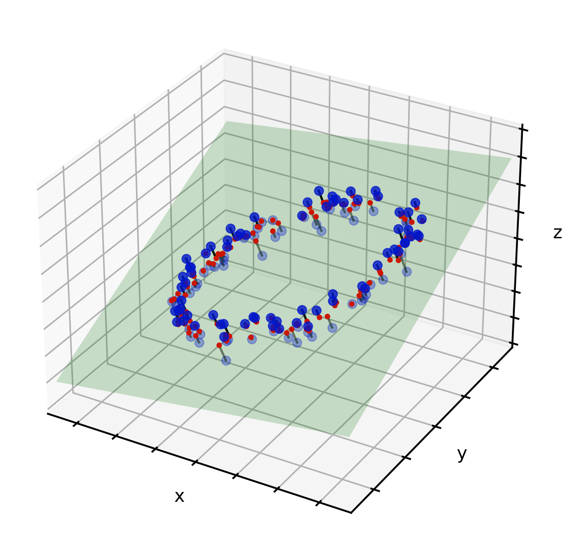
Now that we know the location of all of these shadows on the green plane, we can use a new two-dimensional visualization and plot the points once more.
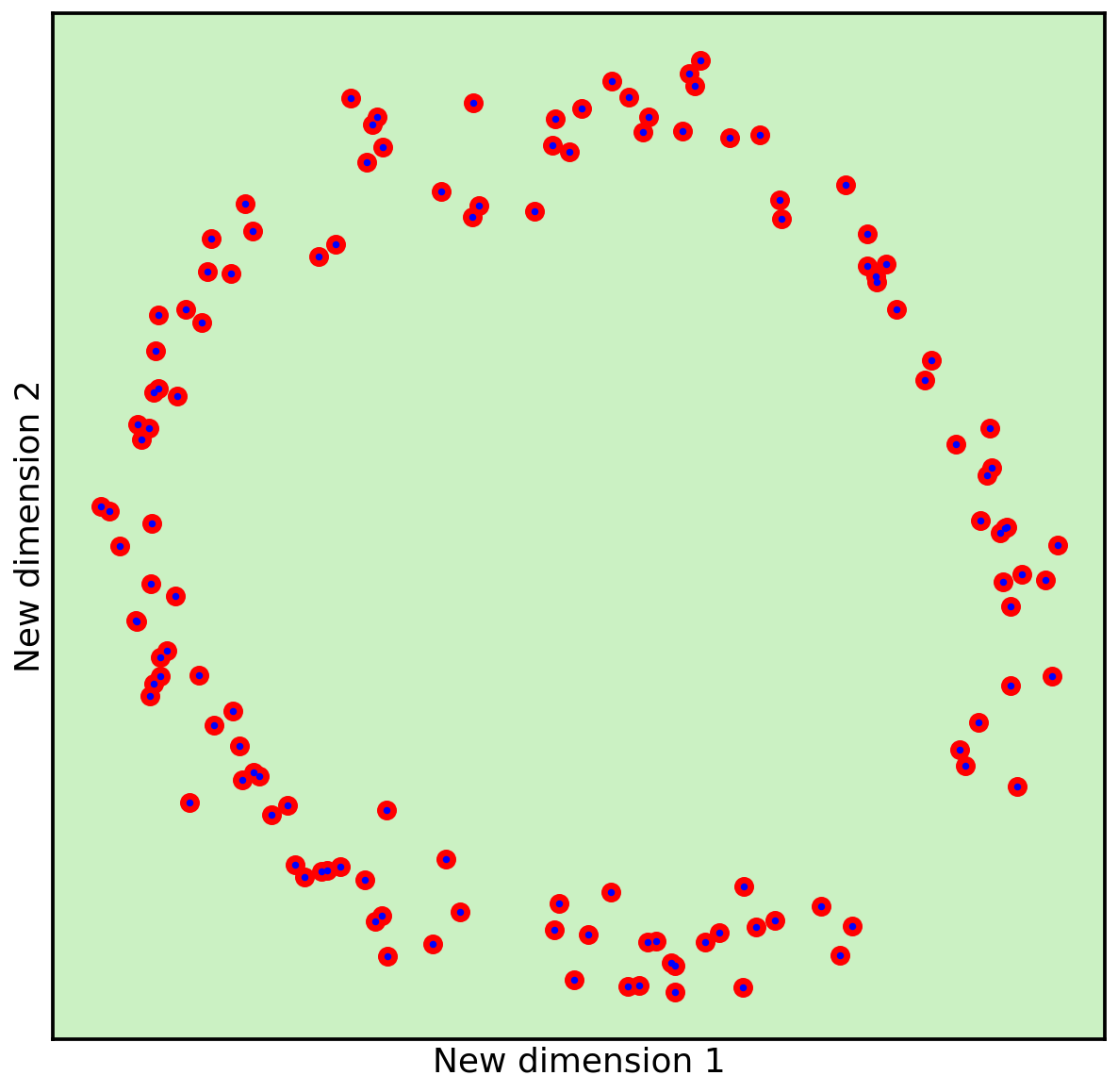
As we can see, the circle is still clearly visible. The only thing lost are the small distances the blue points were away from the green plane. In this case, we can consider that to be noise, as the shape of the circle is preserved.
In summary, because the blue dots in our three-dimensional dataset were laying on a lower-dimensional (green) plane, we were able to project the points down to this lower dimension while still keeping the relevant information that makes up the circle.
Manifolds
In the context of machine learning, a manifold describes an arbitrary surface in high-dimensional space. For example, a crumpled sheet of paper, a donut, or a sphere are all surfaces in a three-dimensional space.
As you see in this example, a manifold surface doesn’t need to be very flat; it can be curvy, twisted, or even have holes. What is important is that even if the overall manifold surface has an irregular shape, at each individual location the surface seems flat. Imagine an insect walking on such a manifold surface - such an insect would believe this curvy surface to actually be flat, similar to the way that we humans perceive the world to be flat even though it is round.
A famous example of such a manifold is the so-called Swiss roll dataset.
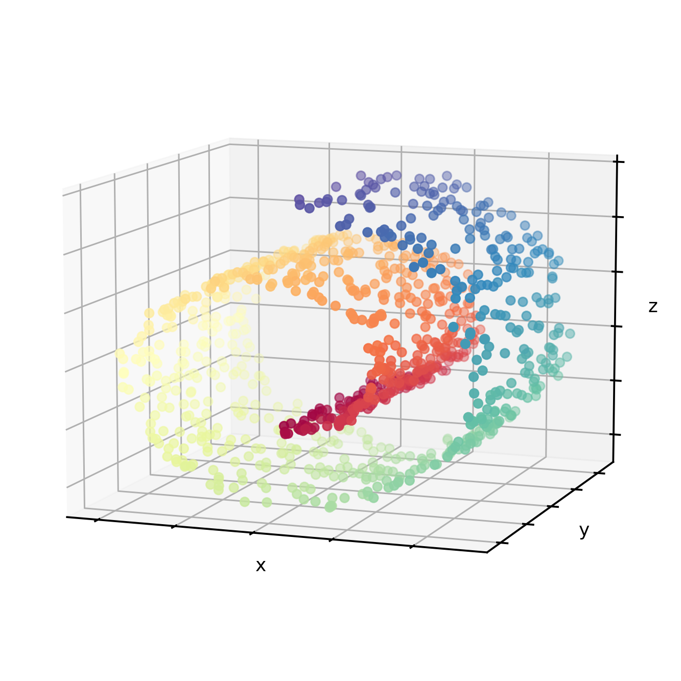
From our superior high-dimensional viewpoint, we can see that the point cloud follows the shape of a Swiss roll and that the color along this curved surface follows the color spectrum.
However, using the aforementioned projection approach wouldn’t work here as there is no flat two-dimensional plane (as in the previous example) to help us to reduce the dimension while keeping the relevant information (i.e. the shape of the Swiss roll). This is where a manifold dimensionality reduction approach can help.
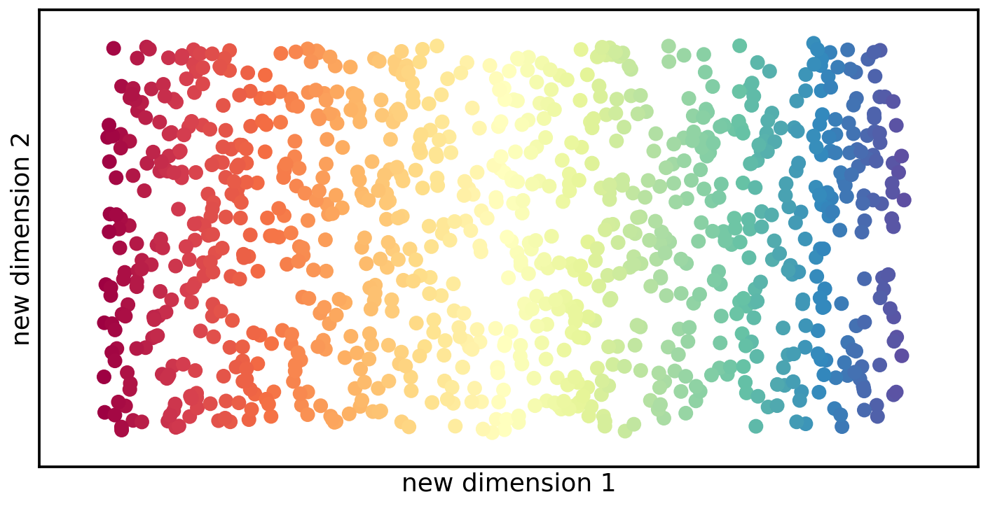
There are multiple ways to find the optimal manifold that would unravel the Swiss roll onto a two-dimensional plane. What all of these approaches have in common is that they try to find the curvy and twisted shape that underlies the point cloud, and unfold and flatten this surface down onto a lower-dimension.
The goal of this unfolding is to keep points that are close to each other in the higher-dimension also close to each other in the lower-dimension – and points that are far away in the higher-dimension also far away in the lower-dimension. The following figure shows one example of how the Swiss roll can be unravelled down to a two-dimensional plane.
Autoencoders
In the context of machine learning, an autoencoder is a specific type of artificial neural network used for unsupervised learning. The architecture of such autoencoder networks can be split into two important parts: an encoder that tries to learn a meaningful low-dimensional representation of the input data; and a decoder that tries to reconstruct the original data from this low-dimensional representation and deliver it as the output data.
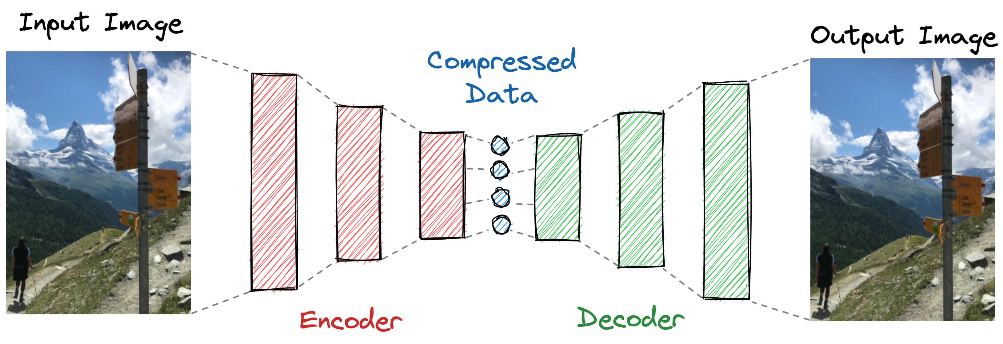
Imagine asking a friend to summarize a three-hour movie they just saw in a five-minute review. Then, after hearing this review, you hire a Hollywood movie crew to try and recreate the full movie based on the information you received from your friend. In this instance, your friend would be the encoder and you would be the decoder.
An initial attempt is certainly bound to fail. But who knows? With time, your friend’s description and your recreation skills will improve and eventually, after decades of training, the final recreation of the movie might be good enough for a naive audience not to notice the difference between the original movie and your version.
In that case, your friend’s five-minute review would seem to be a reasonably good summary of the movie, i.e. a useful compression of the original input data. In other words, the information from the full movie (the information in high-dimension), would be reduced to the much smaller format of a five-minute review (the information in low-dimension).
While a projection or a manifold approach tries to find a coherent surface to reduce the dimensionality of a high-dimensional dataset, an autoencoder doesn’t care about such constraints. Beyond looking for these underlying surfaces, an autoencoder profits from the advantages of neural networks and tries to identify which part of the information in the data can be considered as meaningful, and what can be considered noise – and can therefore be ignored.
Examples of machine-based dimensionality reduction approaches
To further cement our understanding of dimensionality reduction, let’s observe the three different approaches – projection, manifold and autoencoder – in action. For this purpose we will use the Fashion-MNIST dataset. This is a well-known machine learning dataset often used to test new AI models.
The dataset contains 70,000 images of fashion articles from Zalando’s fashion catalog. Each of these 70,000 clothing items belong to one of 10 clothing categories: T-shirt/top, trouser, pullover, dress, coat, sandal, shirt, sneaker, bag, and ankle boot.
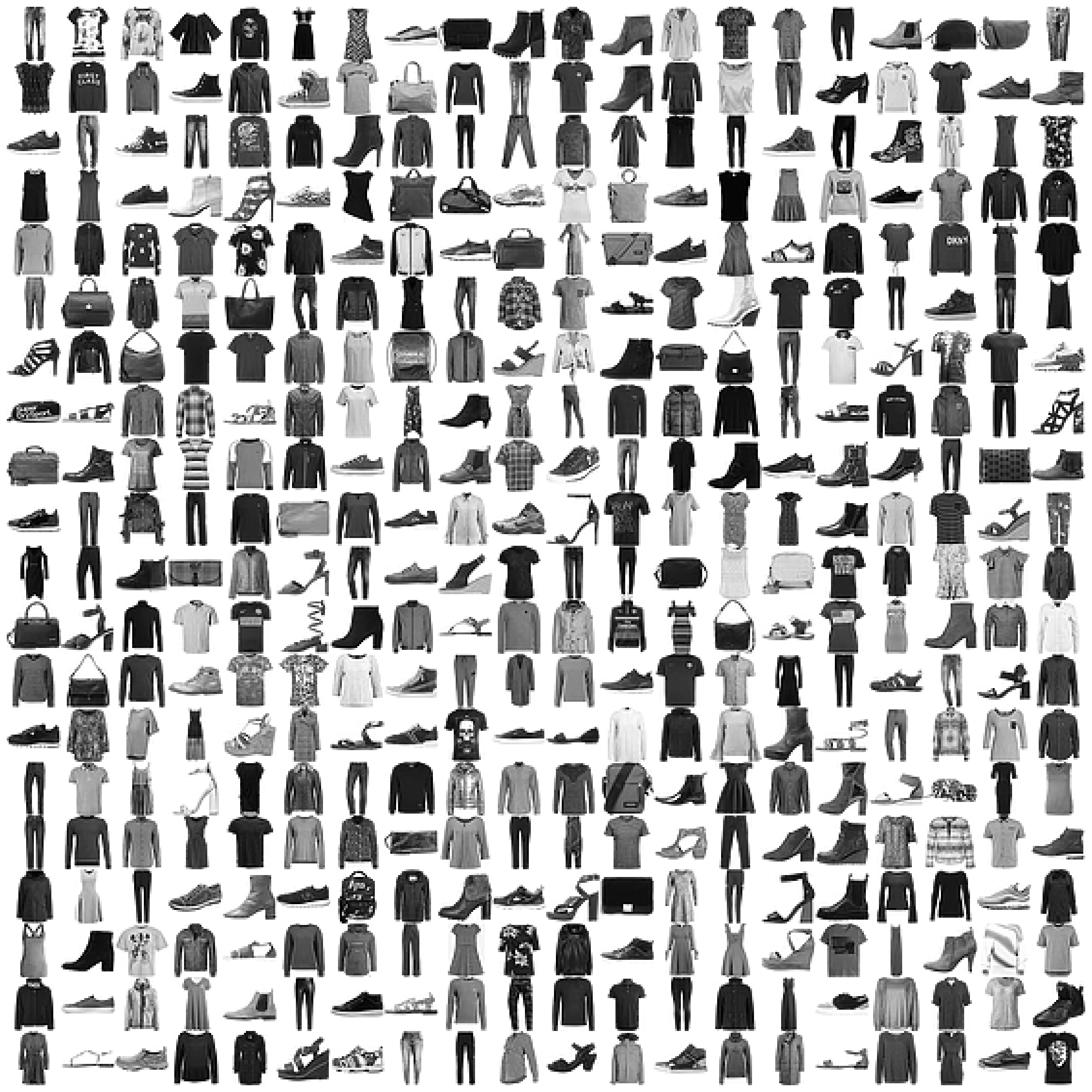
Each item in this dataset is a small black and white picture, with an image resolution of 28x28 pixels. In other words, each image has 784 (28x28 = 784) individual values. Each image can therefore be represented as a point in a 784-point dimensional space. In the following examples we will use these images to see the effect of the different dimensionality reduction approaches.
Dimensionality reduction using projection
One of the most common projection approaches used in machine learning is the so-called principal component analysis, or PCA for short. PCA is a great way to reduce the dimensionality of a dataset by looking for the main characteristics (also called components in this context) that explain most of the information in a dataset. As a consequence, the small nuanced differences between data points are considered as less relevant and are usually dropped for the sake of dimensionality reduction.
The following figure shows the effect of this dimensionality reduction. In the first row, we can see one fashion item from each category in its original form, i.e. when using all 784 dimensions of information. Subsequently, each following row shows what these items would look like if we only used 400, 200, 50, 10 or two of the most relevant dimensions.
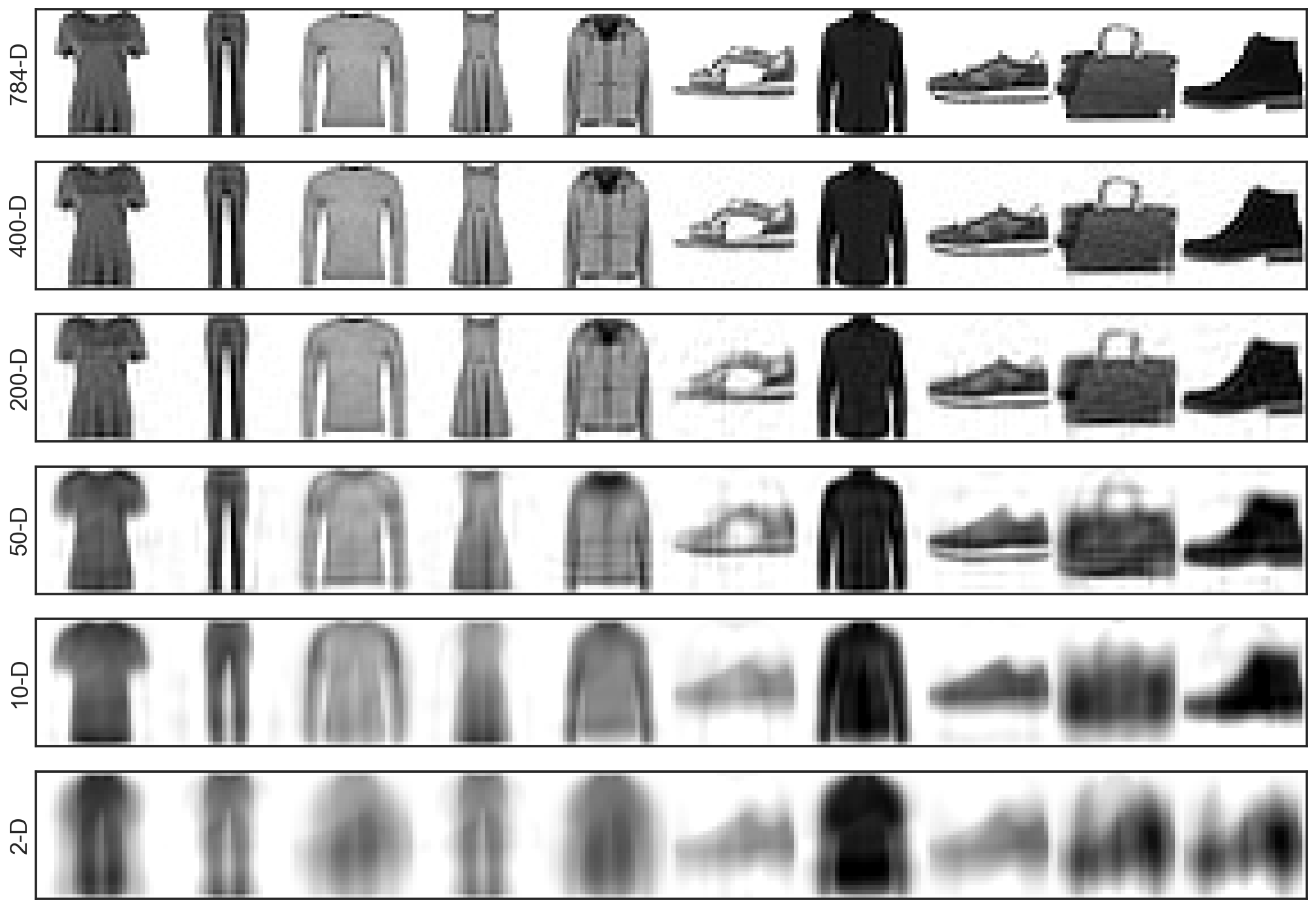
This example accurately illustrates how such a projection approach can be used to reduce the size of the dataset while keeping most of the original information intact. For example, the images in the third row, using only 200 PCA components, still look very much like the original images, but the dataset itself is now only 25% of the original size. This reduction in size can have multiple advantages in the world of machine learning, most notably a speed up in the training of models due to a lower computational demand.
As with all dimensionality reduction approaches, such a projection approach can also be used to visualize high-dimensional data in two-dimension. If we use a projection approach to reduce the 784-dimensional fashion dataset to just two dimensions for example, we would get the following visualization:

Dimensionality reduction using manifolds
When working with data like the fashion dataset, a manifold approach might be an even more powerful dimensionality reduction approach compared to the projection one – not just for reducing the size of the dataset, but also for visualizing the data in two dimensions.
Let’s consider again what the dataset actually represents. Each image is defined by 784 individual pixels, however when we look at this particular dataset, we can see that most images have white corners, show connected lines, have filled out regions and that the objects depicted in the images are more or less shaped like an object from one of the 10 classes.
Keep in mind that this 784-dimensional space contains all 28x28 pixel images that could possibly exist. This high-dimensional space also contains a small image of a grumpy cat, of the EPFL logo, or of your loved ones.
In other words, in contrast to all possible pictures that could ever exist, these 70,000 images from the fashion dataset are actually very much clumped into the same region of this high-dimensional space – i.e. they can be found on one unifying manifold surface.
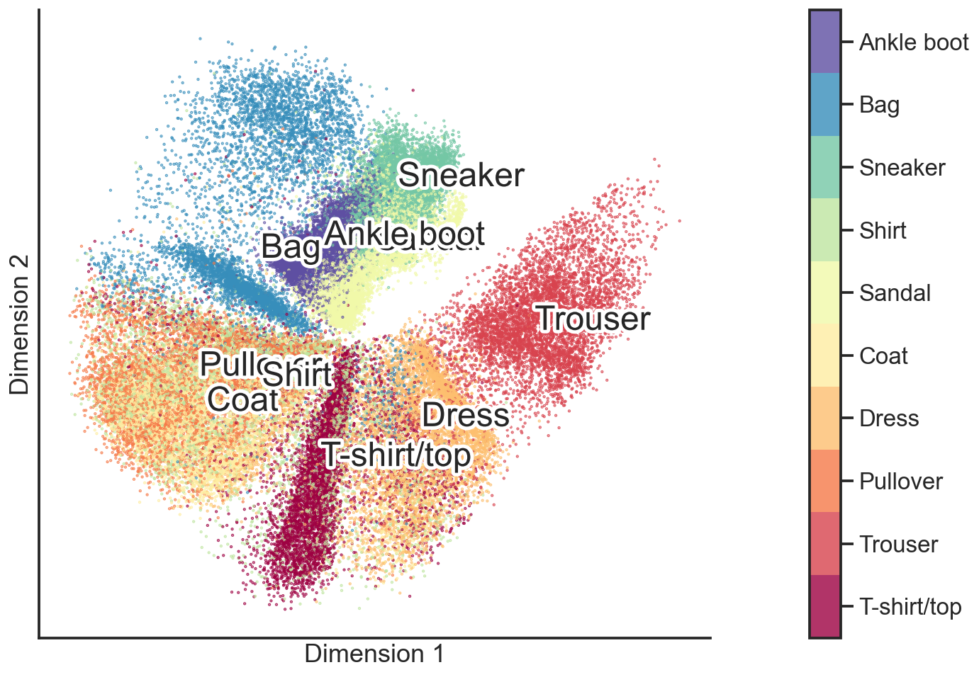
Having said all this, let’s now see what an unsupervised machine learning model trained on the fashion dataset can do. Can this AI find an underlying manifold that can be unravelled and flattened, so that we can visualize the dataset in a two-dimensional figure?
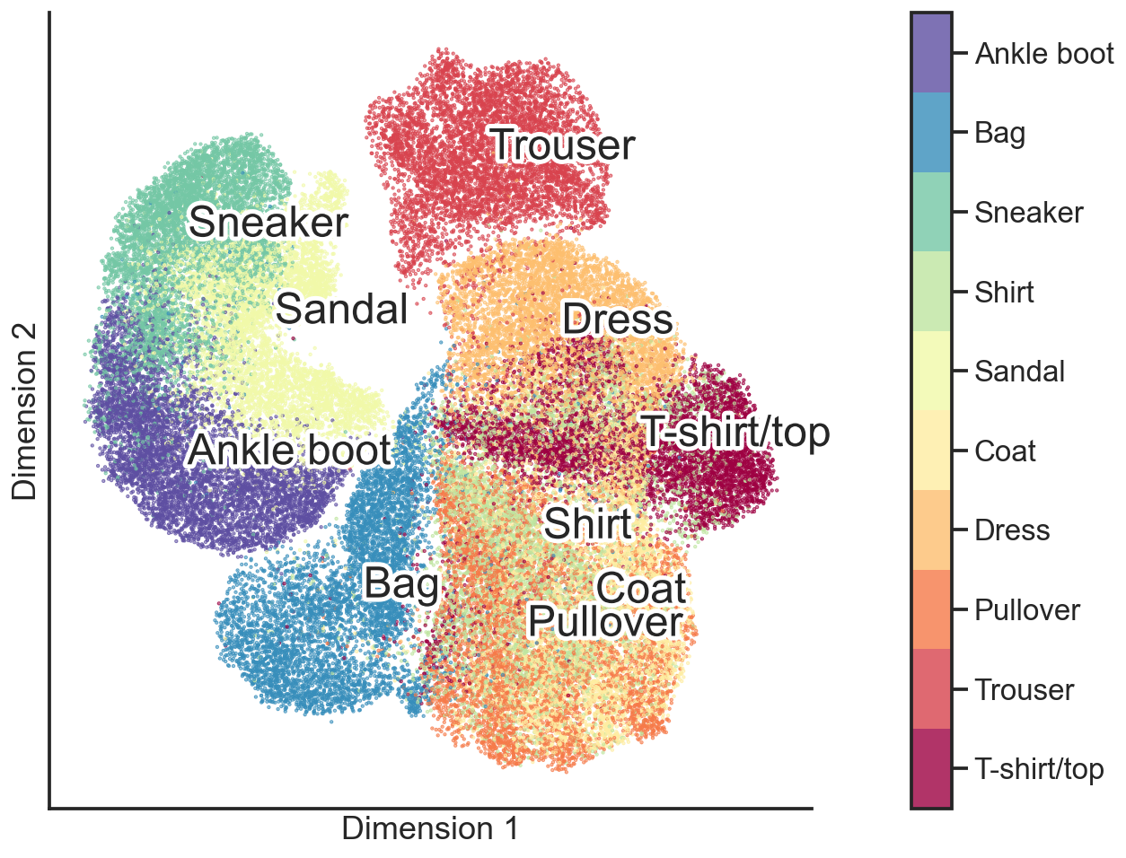
Great, it seems to have worked! The 10 classes are more or less distinct on this flattened two-dimensional manifold. Now what’s even cooler is that we can take any point on this two-dimensional plane and put it back onto the surface in the high-dimensional manifold, thus reverting the dimensionality reduction.
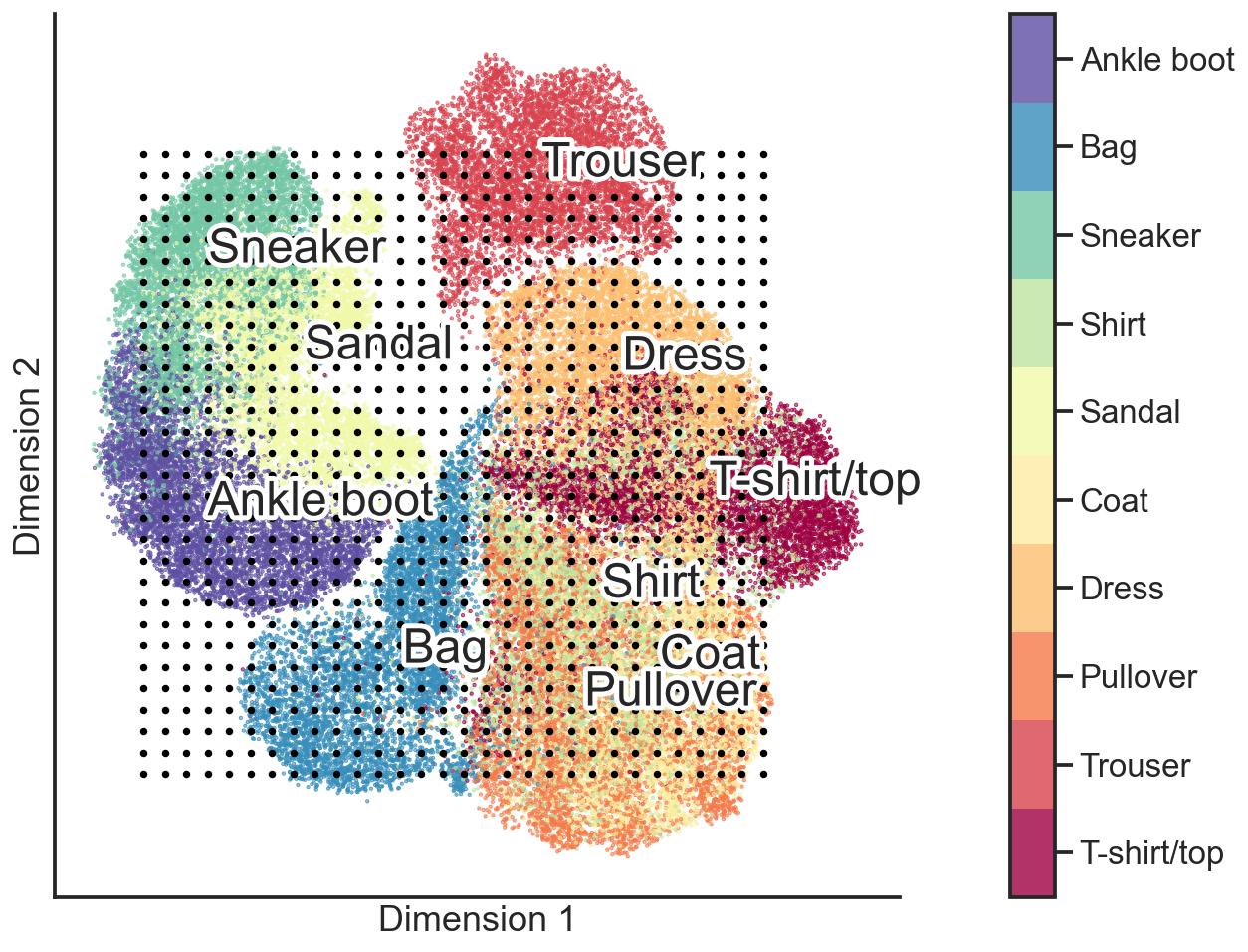
For example, let’s define a grid of points on this two-dimensional plane (the black dots in the figure above) and project them back into the original high-dimensional space with 784-dimensions. Each of the images in the illustration below represents a black dot from the point cloud above.
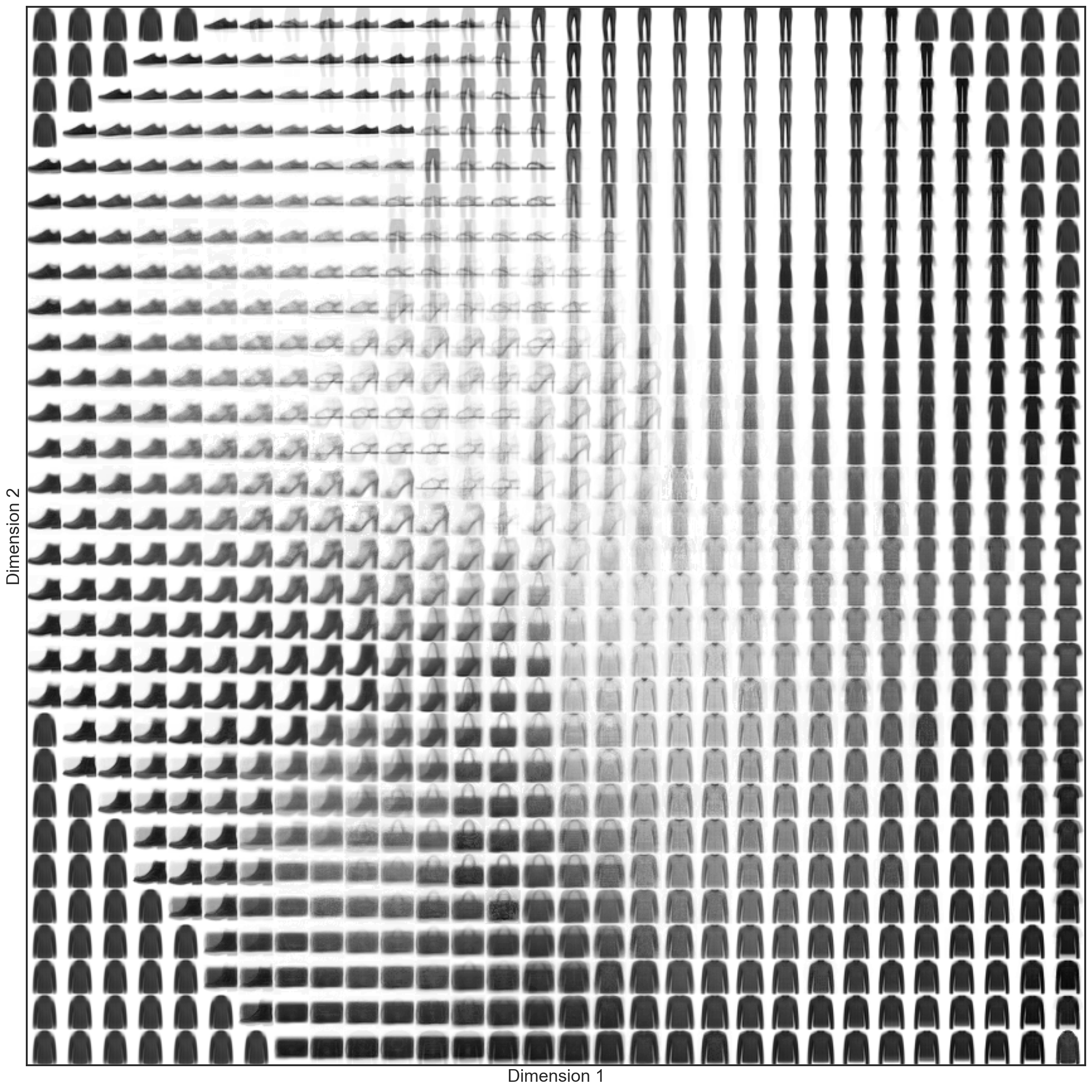
While not every image from this illustration is a realistic depiction of a fashion item, it is nonetheless clear that the AI model has extracted a useful data compression. Specifically, it is able to take an image of a fashion item in this 784-dimensional space and reduce it down to two-dimension. This is a reduction of 99.75% from the original dataset size.
Dimensionality reduction using autoencoders
Last but certainly not least, we will take a quick look at how an autoencoder model would handle this fashion dataset. To briefly recap, an autoencoder model takes the 28x28 sized image as input. During encoding the AI tries to compress the information into only a few dimensions, here into two dimensions. Then during decoding, it tries to unravel this low-dimension information again to re-establish the original image data. The idea is that such an approach allows us to get a meaningful low-dimensional representation of the high-dimensional data.
Once such an autoencoder is trained, we can take the first part of the model (the encoder) and reduce each image from 784-dimensions down to our desired two dimensions. The following image shows what this would look like:
The great thing about autoencoders is that we can now use the second part of the model (the decoder) to recreate any point of this two-dimensional image back into an image with 28x28 pixels. Just like in the manifold example before, we can now put a grid over this two-dimensional figure and ask the model to recreate the corresponding 784-dimensional image. What we get when we do so is this:
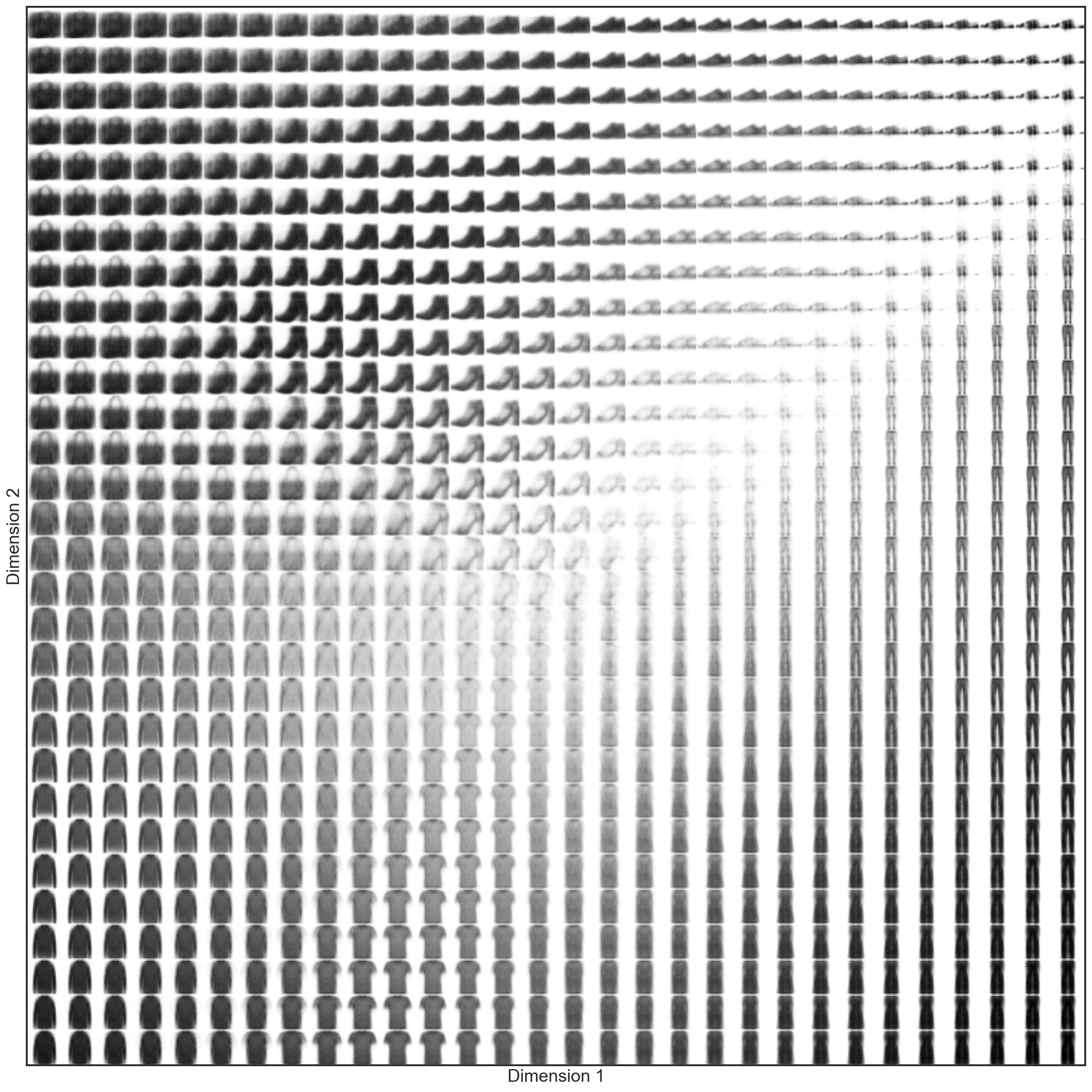
The result of this approach looks very similar to the one we got in the manifold example. But while being able to perform the same tasks as the other two approaches (i.e. reducing the size of a dataset or visualizing big data in two dimensions), autoencoders have one additional unique characteristic: they can also be used to map one high-dimensional version of the dataset to another high-dimensional version of a comparable dataset.
For example, an autoencoder can be set up to take gray images as an input and generate colored images as an output; or take noisy low-resolution images as input and generate high-resolution denoised images; or take holiday photos with a lot of tourists in them as input and generate output images where the tourists are no longer present; and so on…
If the encoder and decoder part are correctly set up – and the data is available – then this kind of model can learn almost any kind of transformation.